Oseltamivir (Patel 2015) • nlmixr2lib

Model and source

#> ℹ parameter labels from comments will be replaced by 'label()'

Citation: Patel K, Rayner CR, Giraudon M, Kamal MA, Morcos PN, Robson R, Kirkpatrick CM. Pharmacokinetics and safety of oseltamivir in patients with end-stage renal disease treated with automated peritoneal dialysis. Br J Clin Pharmacol. 2015;79(4):624-635. doi:10.1111/bcp.12526
Article: https://doi.org/10.1111/bcp.12526
Free full text: https://pmc.ncbi.nlm.nih.gov/articles/PMC4386947/

Patel 2015 gave a single 75 mg oral dose of oseltamivir to ten adults with end-stage renal disease immediately before an aggressive automated peritoneal dialysis (APD) block, then followed oseltamivir and its active metabolite oseltamivir carboxylate in plasma, dialysate and urine for 168 h. The purpose was to work out whether the 75 mg dose is right for these patients, and the model exists to answer that by dose simulation.

The structure is Figure 1 of the paper. Oseltamivir enters a gut compartment with a lag; the fraction F_met = 0.964 is converted to carboxylate by hepatic first pass and passes through an empirical first-pass compartment that releases carboxylate slowly (ka_OC = 0.109 1/h, twelve-fold slower than the prodrug’s own absorption), which is how the model reproduces the roughly 28 h gap the authors observed between the parent and metabolite peaks. The remaining 3.6% is absorbed as unchanged prodrug into a two-compartment parent disposition and converted systemically at CL_pm = 9.63 L/h/70 kg. Carboxylate then leaves a one-compartment disposition by four parallel routes, three of which this study measured directly.

The point of interest is that the dialysate route is split by exchange modality. Cycler-assisted exchanges clear carboxylate at 0.319 L/h/70 kg and ambulatory exchanges at 0.170 L/h/70 kg – a 1.9-fold difference – so the model carries them as two arms gated by the time-varying RRT_CCPD_ACTIVE / RRT_CAPD_ACTIVE session indicators, and the gates alternate as the dialysis schedule cycles. That is what lets the model be re-run under a different APD prescription, which is the whole point of the paper’s simulation section.

ui$props$cmt        # ODE states, in Figure 1's compartment order
#> [1] "depot"              "transit_oselcarb"   "central"           
#> [4] "peripheral1"        "central_oselcarb"   "dialysate_oselcarb"
#> [7] "urine_oselcarb"
ui$props$endpoint   # the four measured outputs
#> NULL

Population

Of 27 patients screened, 10 were enrolled; patient 2 was excluded from the PK analysis for a protocol violation, so the model was fitted to n = 9. Mean age was 52.8 years (range 24-70), 50% were male, and weights spanned 60-92 kg (Table 1). Five patients were anuric and five had residual urine production. Baseline serum creatinine was 320-1461 umol/L. All subjects were on concomitant medication.

Every patient was converted to a standardized APD regimen for the study: three cycler-assisted exchanges of 2.5 L over an 8 h daytime block, then two ambulatory exchanges of 2.0 L over 16 h overnight. This was chosen deliberately as a worst-case high-clearance scenario, not as typical practice.

str(ui$population, max.level = 1)
#> List of 16
#>  $ species       : chr "human"
#>  $ n_subjects    : num 9
#>  $ n_studies     : num 1
#>  $ age_range     : chr "24-70 years"
#>  $ age_median    : chr "mean 52.8 years (Results, Study population)"
#>  $ weight_range  : chr "60-92 kg"
#>  $ weight_median : chr "79 kg (median of the 10 enrolled patients, Table 1)"
#>  $ sex_female_pct: num 50
#>  $ race_ethnicity: Named num [1:4] 20 40 30 10
#>   ..- attr(*, "names")= chr [1:4] "Caucasian" "Pacific Islander" "Indian/African" "Maori"
#>  $ disease_state : chr "End-stage renal disease on stable peritoneal dialysis for at least 3 months, with total Kt/V > 1.7 and a perito"| __truncated__
#>  $ renal_function: chr "Anuric (n = 5) or residual urine production (n = 5; n = 4 in the PK analysis set). Baseline serum creatinine 32"| __truncated__
#>  $ dose_range    : chr "Single 75 mg oral dose of oseltamivir (75000 ug) on day 1, administered immediately before the start of the aut"| __truncated__
#>  $ regions       : chr "New Zealand (two specialist clinical study facilities; ClinicalTrials.gov NCT01556633)."
#>  $ n_observations: chr "Plasma oseltamivir and oseltamivir carboxylate predose and at 0.5, 1.33, 2, 2.5, 3, 4, 5, 6.67, 8, 10, 12, 14, "| __truncated__
#>  $ dialysis      : chr "Standardized aggressive automated peritoneal dialysis: three continuous cycler-assisted (CCPD) exchanges of 2.5"| __truncated__
#>  $ notes         : chr "Of 27 patients screened, 10 were enrolled and all 10 were included in the safety evaluation. Patient 2 was excl"| __truncated__

Two covariates were screened and not retained – serum creatinine and body surface area. That matters for interpreting the model: the paper states that “inclusion of creatinine clearance as a covariate effect did not significantly improve the model”, and the Discussion is blunter still – residual renal clearance “was not predicted by serum creatinine measurement or estimated creatinine clearance”. So ANURIA is the only renal covariate the model can use, and the 117% between-subject variability on the renal arm is genuinely unexplained rather than merely unmodelled.

names(ui$covariatesDataExcluded)
#> [1] "CREAT" "BSA"

Source trace

Every value below is also carried as an in-file comment beside its ini() entry in inst/modeldb/specificDrugs/Patel_2015_oseltamivir.R.

Parameter / equation	Value	Source location
Model topology (7 compartments, all flux arrows)	n/a	Figure 1
`logitfm` (F_met)	0.964, logit 3.287572	Table 2, Absorption
`lka` (ka_OP)	1.36 1/h	Table 2, Absorption
`ltlag` (Alag_OP)	0.485 h	Table 2, Absorption
`lka_oselcarb` (ka_OC)	0.109 1/h	Table 2, Absorption
`lcl_met` (CL_pm)	9.63 L/h/70 kg	Table 2, Oseltamivir disposition
`lvc` (Vc_OP)	16.7 L/70 kg	Table 2, Oseltamivir disposition
`lq` (CL_D)	6.80 L/h/70 kg	Table 2, Oseltamivir disposition
`lvp` (Vp_OP)	307 L/70 kg	Table 2, Oseltamivir disposition
`lvc_oselcarb` (Vc_OC)	32.8 L/70 kg, FIXED	Table 2 + Methods (fixed from Rayner et al., ref 18)
`lcl_ccpd_oselcarb`	0.319 L/h/70 kg	Table 2, carboxylate disposition
`lcl_capd_oselcarb`	0.170 L/h/70 kg	Table 2, carboxylate disposition
`lcl_renal_oselcarb`	0.736 L/h/70 kg	Table 2, carboxylate disposition
`lcl_other_oselcarb`	0.319 L/h/70 kg	Table 2, carboxylate disposition
All BSV terms	7.70-147% CV	Table 2, BSV (CV%) column
`propSd` (parent plasma)	35.9 CV%	Table 2, Residual error
`addSd_oselcarb`	73.1 ug/L	Table 2, Residual error
`propSd`/`addSd_dialysateOselcarb`	14.0 CV%, 11.6 ug	Table 2, Residual error
`propSd_urineOselcarb`	35.5 CV%	Table 2, Residual error
Amount / concentration units	ug, ug/L	Table 2 footnote (dagger)
APD schedule (CCPD 8 h / CAPD 16 h)	n/a	Methods “Treatments” + Table 3 footnote (section)
Renal strata for simulation	0.289 (45% BSV), 2.50 (10% BSV)	Table 3 footnotes (pilcrow, double asterisk)
Target exposures	AUC0-120 31820 ug.h/L, C120 170 ug/L	Methods “Monte Carlo simulations” (Rayner et al., ref 18)
`e_wt_cl`, `e_wt_vc`	0.75, 1.0 (not printed)	see Assumptions below

Virtual cohort and simulation helpers

Doses are in micrograms and concentrations in ug/L (= ng/mL), the units the source model was fitted in, so the 75 mg clinical dose is 75000.

The APD schedule enters as the two time-varying session gates. The three prescriptions the paper simulated (Table 3 footnotes and Methods) are encoded below as functions of clock time within each 24 h cycle.

# Patel 2015 Methods / Table 3 footnotes. Each returns the CCPD gate; the CAPD
# gate is supplied separately because two of the three regimens include dry
# time, during which BOTH gates are 0 and only the renal and other routes clear.
apd_gates <- function(time, regimen) {
  tday <- time - 24 * floor(time / 24)
  switch(regimen,
    # (iii) the regimen actually studied: 3 CCPD exchanges over 8 h daytime,
    # then 2 CAPD exchanges over 16 h overnight. No dry time.
    "Intensive APD" = list(ccpd = as.numeric(tday <  8),
                           capd = as.numeric(tday >= 8)),
    # (i) CAPD only: 3 exchanges over 15 h during the day, then one 9 h
    # exchange overnight -- continuous ambulatory cover, no cycler.
    "CAPD only"     = list(ccpd = rep(0, length(tday)),
                           capd = rep(1, length(tday))),
    # (ii) intermediate: one CAPD exchange over 10 h, a 2 h break, three CCPD
    # sessions over 9 h, then a 3 h break.
    "Intermediate APD" = list(ccpd = as.numeric(tday >= 12 & tday < 21),
                              capd = as.numeric(tday <  10)),
    stop("unknown regimen: ", regimen)
  )
}

# Patel 2015 Table 3 renal strata. The anuric arm switches the renal route off
# via ANURIA; the two urine-producing arms replace the model's population
# estimate (0.736 L/h/70 kg, 117% BSV) with the paper's post-hoc subgroup
# medians and BSVs, which is what its own simulations used.
renal_strata <- list(
  "Anuric"     = list(anuria = 1, cl = NA_real_, cv = NA_real_),
  "Low urine"  = list(anuria = 0, cl = 0.289,    cv = 0.45),
  "High urine" = list(anuria = 0, cl = 2.50,     cv = 0.10)
)

stratum_model <- function(stratum) {
  s <- renal_strata[[stratum]]
  if (s$anuria == 1L) return(readModelDb("Patel_2015_oseltamivir"))
  rxode2::ini(readModelDb("Patel_2015_oseltamivir"),
              lcl_renal_oselcarb    =  log(s$cl),
              etalcl_renal_oselcarb ~  log(1 + s$cv^2))
}

# `set.seed()` seeds R's RNG, NOT rxode2's simulation RNG, and rxode2's streams
# are partitioned per solver thread -- so this cohort differs between a 2-core
# CI runner and a 16-thread workstation and no seed can make them agree. Every
# assertion below is therefore written on a centre or a robust bound, never on
# an extreme, a sign, or an exact value. See pattern 12 of
# .claude/skills/extract-literature-model/references/known-vignette-failure-patterns.md
set.seed(20150401)

# 150 subjects per arm. The paper simulated 1000; 150 keeps the Monte Carlo
# standard error at or below ~4 percentage points on a probability, which is
# well inside the tolerances asserted below, and keeps the render fast.
N_PER_ARM <- 150L

# Observation grid: dense through absorption and the metabolite peak, coarser
# through the long terminal phase. Fine enough that trapezoidal AUC0-120 is
# accurate to well under 1%.
OBS_GRID <- sort(unique(c(seq(0, 24, by = 0.5), seq(24, 168, by = 2))))

# Build one arm as a self-contained event table. `id_offset` keeps IDs disjoint
# across bind_rows()-ed arms -- duplicate IDs are silently merged by rxSolve
# into one subject receiving the summed dose.
make_arm <- function(n, dose_ug, dose_times, stratum, regimen,
                     wt = 70, grid = OBS_GRID, id_offset = 0L) {
  subj <- tibble(
    id      = id_offset + seq_len(n),
    WT      = wt,
    ANURIA  = renal_strata[[stratum]]$anuria,
    stratum = stratum,
    regimen = regimen,
    arm     = paste0(stratum, " | ", dose_ug[1] / 1000, " mg | ", regimen)
  )
  dos <- tidyr::expand_grid(id = subj$id, k = seq_along(dose_ug)) |>
    transmute(id, time = dose_times[k], amt = dose_ug[k],
              evid = 1L, cmt = "depot", dvid = NA_integer_)
  # dvid = 1L on EVERY observation row: the model has four `~` endpoints, so
  # rxode2 needs a dvid mapping, and dvid = 1L returns all four columns.
  obs <- tidyr::expand_grid(id = subj$id, time = grid) |>
    transmute(id, time, amt = NA_real_, evid = 0L,
              cmt = NA_character_, dvid = 1L)
  g <- bind_rows(dos, obs) |>
    left_join(subj, by = "id") |>
    arrange(id, time, desc(evid))
  gates <- apd_gates(g$time, regimen)
  g$RRT_CCPD_ACTIVE <- gates$ccpd
  g$RRT_CAPD_ACTIVE <- gates$capd
  g
}

# `useLinCmt = FALSE` is required: rxSolve.rxUi's default ODE -> linCmt
# auto-conversion corrupts the dvid -> cmt mapping for multi-output models of
# this shape (pattern 5b of known-vignette-failure-patterns.md).
solve_arm <- function(events, stratum) {
  rxode2::rxSolve(
    stratum_model(stratum), events = events,
    keep = c("stratum", "regimen", "arm", "WT"),
    useLinCmt = FALSE, returnType = "data.frame"
  ) |>
    filter(!is.na(Cc_oselcarb))
}

Structural checks

These are typical-value (deterministic) quantities, so they are asserted exactly rather than with a tolerance.

typ <- function(stratum, regimen = "Intensive APD", dose = 75000, wt = 70) {
  ev <- make_arm(1L, dose, 0, stratum, regimen, wt = wt)
  rxode2::rxSolve(rxode2::zeroRe(stratum_model(stratum)), events = ev,
                  useLinCmt = FALSE, returnType = "data.frame",
                  atol = 1e-10, rtol = 1e-8) |>
    filter(!is.na(Cc_oselcarb))
}
tv <- typ("Anuric")
#> ℹ parameter labels from comments will be replaced by 'label()'
#> ℹ omega/sigma items treated as zero: 'etalogitfm', 'etalka', 'etaltlag', 'etalvc', 'etalvc_oselcarb', 'etalcl_ccpd_oselcarb', 'etalcl_capd_oselcarb', 'etalcl_renal_oselcarb', 'etalcl_other_oselcarb'

# 1. F_met is bounded in (0, 1) for every subject. This is why the model
#    carries F_met on the logit scale: Table 2's 16.9% CV read as an
#    exponential eta on 0.964 would put F_met above 1 for ~41% of subjects and
#    drive the parent central compartment negative.
fm_cohort <- solve_arm(make_arm(N_PER_ARM, 75000, 0, "Anuric", "Intensive APD"), "Anuric")
#> ℹ parameter labels from comments will be replaced by 'label()'
stopifnot(
  all(fm_cohort$fm > 0), all(fm_cohort$fm < 1),
  # 2. and no negative parent concentration anywhere in the cohort
  all(fm_cohort$Cc >= 0), all(fm_cohort$Cc_oselcarb >= 0)
)

# 3. Mass conservation across the gut split: the two absorption arms must sum
#    to ka * depot, so cumulative dialysate + urine can never exceed the dose.
stopifnot(max(tv$dialysateOselcarb + tv$urineOselcarb) <= 75000)

# 4. The parent peaks early and the metabolite late -- the paper's motivating
#    observation. Parent tmax follows directly from ka_OP and the lag.
tmax_op <- tv$time[which.max(tv$Cc)]
tmax_oc <- tv$time[which.max(tv$Cc_oselcarb)]
stopifnot(tmax_op > 0.485, tmax_op < 3, tmax_oc > 12, tmax_oc < 30)

# 5. Parent oseltamivir is rapidly removed by first-pass metabolism: by 10 h
#    it has fallen to under 5% of its peak (Results: "Oseltamivir was rapidly
#    removed from the plasma via first-pass metabolism"). Asserted as a
#    fraction of peak rather than against the 1.00 ug/L assay LOQ -- the model
#    sustains a shallow tail just above the LOQ, which is recorded as a
#    deviation below.
cc10_frac <- tv$Cc[which.min(abs(tv$time - 10))] / max(tv$Cc)
stopifnot(cc10_frac < 0.05)

tibble(
  check = c("parent tmax (h)", "metabolite tmax (h)",
            "parent Cc at 10 h, fraction of peak",
            "parent Cc at 10 h (ug/L)", "F_met range across cohort"),
  value = c(sprintf("%.2f", tmax_op), sprintf("%.2f", tmax_oc),
            sprintf("%.4f", cc10_frac),
            sprintf("%.3f", tv$Cc[which.min(abs(tv$time - 10))]),
            sprintf("%.4f - %.4f", min(fm_cohort$fm), max(fm_cohort$fm)))
) |>
  knitr::kable(caption = "Deterministic structural checks.")

Deterministic structural checks.
check	value
parent tmax (h)	1.50
metabolite tmax (h)	22.50
parent Cc at 10 h, fraction of peak	0.0206
parent Cc at 10 h (ug/L)	1.414
F_met range across cohort	0.9454 - 0.9770

Replicating Figure 2 – plasma profiles

# Replicates Figure 2A/2B of Patel 2015: mean plasma oseltamivir (A) and
# oseltamivir carboxylate (B) on a log scale after a single 75 mg dose. The
# cohort mixes anuric and urine-producing patients as the study did (5:4).
fig2 <- bind_rows(
  make_arm(84L, 75000, 0, "Anuric",    "Intensive APD", id_offset =   0L),
  make_arm(66L, 75000, 0, "Low urine", "Intensive APD", id_offset = 200L)
)
stopifnot(!anyDuplicated(unique(fig2[, c("id", "time", "evid")])))

fig2_sim <- bind_rows(
  solve_arm(filter(fig2, stratum == "Anuric"),    "Anuric"),
  solve_arm(filter(fig2, stratum == "Low urine"), "Low urine")
)
#> ℹ parameter labels from comments will be replaced by 'label()'
#> ℹ change initial estimate of `lcl_renal_oselcarb` to `-1.2413285908697`
#> ℹ change initial estimate of `etalcl_renal_oselcarb` to `0.184402722997779`

fig2_sim |>
  select(time, Oseltamivir = Cc, `Oseltamivir carboxylate` = Cc_oselcarb) |>
  pivot_longer(-time, names_to = "analyte", values_to = "conc") |>
  filter(conc > 0.1) |>
  group_by(analyte, time) |>
  summarise(Q05 = quantile(conc, 0.05), Q50 = median(conc),
            Q95 = quantile(conc, 0.95), .groups = "drop") |>
  ggplot(aes(time, Q50)) +
  geom_ribbon(aes(ymin = Q05, ymax = Q95), alpha = 0.2) +
  geom_line(linewidth = 0.7) +
  facet_wrap(~analyte, scales = "free_y") +
  scale_x_continuous(breaks = c(0, 24, 48, 72, 96, 120, 144, 168)) +
  scale_y_log10() +
  labs(x = "Time (h)", y = "Plasma concentration (ug/L)",
       caption = paste("Replicates Figure 2A/2B of Patel 2015.",
                       "Median with 5th-95th percentile band."))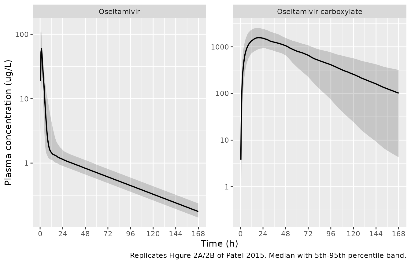

The two panels show the feature the model was built for: the prodrug is gone within about 10 h while the metabolite is still quantifiable at 168 h.

Replicating Figure 3 – dialysate and urine recovery

# Replicates Figure 3C/3D of Patel 2015: cumulative oseltamivir carboxylate
# recovered in dialysate (C) and urine (D). The step pattern in the dialysate
# curve is the CCPD/CAPD gate alternating -- the cycler block clears 1.9-fold
# faster than the ambulatory block.
fig2_sim |>
  select(time, stratum, Dialysate = dialysateOselcarb, Urine = urineOselcarb) |>
  pivot_longer(c(Dialysate, Urine), names_to = "matrix", values_to = "amt") |>
  group_by(stratum, matrix, time) |>
  summarise(Q50 = median(amt), .groups = "drop") |>
  ggplot(aes(time, Q50 / 1000, colour = stratum)) +
  geom_line(linewidth = 0.7) +
  facet_wrap(~matrix) +
  scale_x_continuous(breaks = c(0, 24, 48, 72, 96, 120, 144, 168)) +
  labs(x = "Time (h)", y = "Cumulative recovery (mg)", colour = "Renal stratum",
       caption = paste("Replicates Figure 3C/3D of Patel 2015.",
                       "Median cumulative amount; 75 mg single dose."))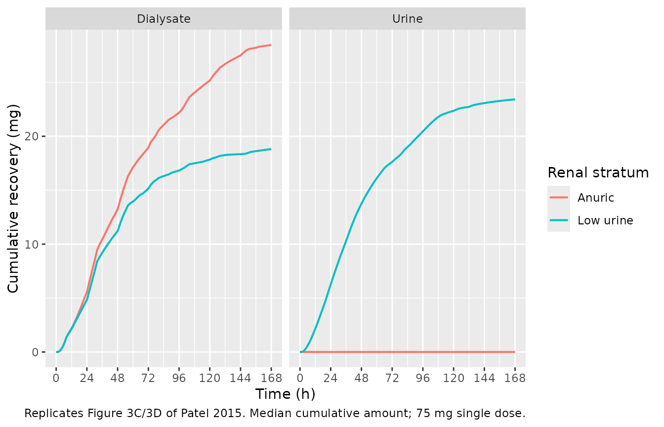

Note that the model reproduces the paper’s central clinical finding directly: in urine producers the renal route dominates and dialysate recovery falls, which is why those patients under-attain the target exposure.

APD regimen comparison

The paper simulated three prescriptions and concluded that “simulated exposures were highest for CAPD only and lowest for the present intensive CAPD/CCPD combination, although only minor differences were observed”. These are typical-value predictions, so the ordering is deterministic and can be asserted strictly.

auc_to <- function(d, end = 120) {
  s <- filter(d, time <= end)
  sum(diff(s$time) * (head(s$Cc_oselcarb, -1) + tail(s$Cc_oselcarb, -1)) / 2)
}
reg_tab <- tibble(regimen = c("CAPD only", "Intermediate APD", "Intensive APD")) |>
  rowwise() |>
  mutate(d = list(typ("Anuric", regimen))) |>
  mutate(`AUC0-120 (ug.h/L)` = auc_to(d), `C120 (ug/L)` = d$Cc_oselcarb[which.min(abs(d$time - 120))]) |>
  ungroup() |>
  select(-d)
#> ℹ parameter labels from comments will be replaced by 'label()'
#> ℹ omega/sigma items treated as zero: 'etalogitfm', 'etalka', 'etaltlag', 'etalvc', 'etalvc_oselcarb', 'etalcl_ccpd_oselcarb', 'etalcl_capd_oselcarb', 'etalcl_renal_oselcarb', 'etalcl_other_oselcarb'
#> ℹ parameter labels from comments will be replaced by 'label()'
#> ℹ omega/sigma items treated as zero: 'etalogitfm', 'etalka', 'etaltlag', 'etalvc', 'etalvc_oselcarb', 'etalcl_ccpd_oselcarb', 'etalcl_capd_oselcarb', 'etalcl_renal_oselcarb', 'etalcl_other_oselcarb'
#> ℹ parameter labels from comments will be replaced by 'label()'
#> ℹ omega/sigma items treated as zero: 'etalogitfm', 'etalka', 'etaltlag', 'etalvc', 'etalvc_oselcarb', 'etalcl_ccpd_oselcarb', 'etalcl_capd_oselcarb', 'etalcl_renal_oselcarb', 'etalcl_other_oselcarb'

# The paper's stated ordering: CAPD only > intermediate > intensive.
stopifnot(
  reg_tab$`AUC0-120 (ug.h/L)`[1] > reg_tab$`AUC0-120 (ug.h/L)`[2],
  reg_tab$`AUC0-120 (ug.h/L)`[2] > reg_tab$`AUC0-120 (ug.h/L)`[3],
  # "only minor differences": realised spread is 5.7% of the largest exposure.
  # Deterministic, so bounded tightly; 15% still admits rounding but breaks if
  # a gate schedule or a dialysate clearance is mis-encoded.
  diff(range(reg_tab$`AUC0-120 (ug.h/L)`)) / max(reg_tab$`AUC0-120 (ug.h/L)`) < 0.15
)
reg_tab |>
  dplyr::rename("APD regimen" = regimen) |>
  knitr::kable(digits = 0, caption = paste(
    "Typical-value exposures for an anuric 70 kg patient after a single 75 mg",
    "dose under the three APD prescriptions of Patel 2015 (Methods, Monte",
    "Carlo simulations). Ordering reproduces the paper's claim."))

Typical-value exposures for an anuric 70 kg patient after a single 75 mg dose under the three APD prescriptions of Patel 2015 (Methods, Monte Carlo simulations). Ordering reproduces the paper’s claim.
APD regimen	AUC0-120 (ug.h/L)	C120 (ug/L)
CAPD only	122473	453
Intermediate APD	118219	407
Intensive APD	115453	391

Replicating Table 3 – probability of target attainment

This is the strongest available gate: Table 3 reports simulated attainment probabilities over a dose x renal-stratum grid against two fixed historical targets, so reproducing it consumes no free parameters.

TARGET_AUC  <- 31820   # ug.h/L, Methods (Rayner et al., ref 18)
TARGET_C120 <- 170     # ug/L

pta_grid <- tidyr::expand_grid(
  stratum = c("Anuric", "Low urine", "High urine"),
  dose_mg = c(75, 60, 45, 30)
)

pta <- pta_grid |>
  mutate(k = row_number()) |>
  rowwise() |>
  mutate(res = list({
    ev <- make_arm(N_PER_ARM, dose_mg * 1000, 0, stratum, "Intensive APD",
                   grid = OBS_GRID[OBS_GRID <= 120], id_offset = 1000L * k)
    solve_arm(ev, stratum) |>
      group_by(id) |>
      summarise(auc120 = sum(diff(time) * (head(Cc_oselcarb, -1) +
                                           tail(Cc_oselcarb, -1)) / 2),
                c120 = Cc_oselcarb[which.min(abs(time - 120))],
                .groups = "drop") |>
      summarise(pta_auc = mean(auc120 >= TARGET_AUC),
                pta_c120 = mean(c120 >= TARGET_C120))
  })) |>
  tidyr::unnest(res) |>
  ungroup() |>
  select(stratum, dose_mg, pta_auc, pta_c120)
#> ℹ parameter labels from comments will be replaced by 'label()'
#> ℹ change initial estimate of `lcl_renal_oselcarb` to `-1.2413285908697`
#> ℹ change initial estimate of `etalcl_renal_oselcarb` to `0.184402722997779`
#> ℹ parameter labels from comments will be replaced by 'label()'
#> ℹ change initial estimate of `lcl_renal_oselcarb` to `-1.2413285908697`
#> ℹ change initial estimate of `etalcl_renal_oselcarb` to `0.184402722997779`
#> ℹ parameter labels from comments will be replaced by 'label()'
#> ℹ change initial estimate of `lcl_renal_oselcarb` to `-1.2413285908697`
#> ℹ change initial estimate of `etalcl_renal_oselcarb` to `0.184402722997779`
#> ℹ parameter labels from comments will be replaced by 'label()'
#> ℹ change initial estimate of `lcl_renal_oselcarb` to `-1.2413285908697`
#> ℹ change initial estimate of `etalcl_renal_oselcarb` to `0.184402722997779`
#> ℹ parameter labels from comments will be replaced by 'label()'
#> ℹ change initial estimate of `lcl_renal_oselcarb` to `0.916290731874155`
#> ℹ change initial estimate of `etalcl_renal_oselcarb` to `0.00995033085316809`
#> ℹ parameter labels from comments will be replaced by 'label()'
#> ℹ change initial estimate of `lcl_renal_oselcarb` to `0.916290731874155`
#> ℹ change initial estimate of `etalcl_renal_oselcarb` to `0.00995033085316809`
#> ℹ parameter labels from comments will be replaced by 'label()'
#> ℹ change initial estimate of `lcl_renal_oselcarb` to `0.916290731874155`
#> ℹ change initial estimate of `etalcl_renal_oselcarb` to `0.00995033085316809`
#> ℹ parameter labels from comments will be replaced by 'label()'
#> ℹ change initial estimate of `lcl_renal_oselcarb` to `0.916290731874155`
#> ℹ change initial estimate of `etalcl_renal_oselcarb` to `0.00995033085316809`

# Patel 2015 Table 3, "Initial simulation" column (the regimen studied).
published <- tibble::tribble(
  ~stratum,     ~dose_mg, ~pub_auc, ~pub_c120,
  "Anuric",     75,       1.000,    0.974,
  "Anuric",     60,       1.000,    0.957,
  "Anuric",     45,       1.000,    0.929,
  "Anuric",     30,       0.973,    0.773,
  "Low urine",  75,       1.000,    0.674,
  "Low urine",  60,       1.000,    0.547,
  "Low urine",  45,       0.998,    0.348,
  "Low urine",  30,       0.773,    0.065,
  "High urine", 75,       0.194,    0.000,
  "High urine", 60,       0.035,    0.000,
  "High urine", 45,       0.000,    0.000,
  "High urine", 30,       0.000,    0.000
)

cmp <- left_join(published, pta, by = c("stratum", "dose_mg")) |>
  mutate(d_auc = pta_auc - pub_auc, d_c120 = pta_c120 - pub_c120)

cmp |>
  transmute(
    "Renal stratum"        = stratum,
    "Dose (mg)"            = dose_mg,
    "AUC PTA published"    = pub_auc,
    "AUC PTA simulated"    = round(pta_auc, 3),
    "C120 PTA published"   = pub_c120,
    "C120 PTA simulated"   = round(pta_c120, 3)
  ) |>
  knitr::kable(caption = paste(
    "Replicates Table 3 (Initial simulation column) of Patel 2015:",
    "probability of attaining AUC0-120 >= 31820 ug.h/L or C120 >= 170 ug/L",
    "after a single oral dose under the intensive APD regimen."))

Replicates Table 3 (Initial simulation column) of Patel 2015: probability of attaining AUC0-120 >= 31820 ug.h/L or C120 >= 170 ug/L after a single oral dose under the intensive APD regimen.
Renal stratum	Dose (mg)	AUC PTA published	AUC PTA simulated	C120 PTA published	C120 PTA simulated
Anuric	75	1.000	1.000	0.974	0.900
Anuric	60	1.000	1.000	0.957	0.827
Anuric	45	1.000	1.000	0.929	0.787
Anuric	30	0.973	0.960	0.773	0.440
Low urine	75	1.000	1.000	0.674	0.433
Low urine	60	1.000	1.000	0.547	0.320
Low urine	45	0.998	0.973	0.348	0.147
Low urine	30	0.773	0.560	0.065	0.007
High urine	75	0.194	0.000	0.000	0.000
High urine	60	0.035	0.000	0.000	0.000
High urine	45	0.000	0.000	0.000	0.000
High urine	30	0.000	0.000	0.000	0.000

# AUC attainment is the gated quantity. Realised mean |difference| 0.042-0.046
# across 1 / 2 / 4 / 16 solver threads, so 0.10 has real headroom while still
# breaking on a mis-transcribed clearance, dose or unit -- any of which move
# every cell by tens of points.
stopifnot(mean(abs(cmp$d_auc)) < 0.10)

# The qualitative conclusions the paper draws from this table must hold.
stopifnot(
  # 75 mg attains the AUC target in anuric and low-urine patients ...
  cmp$pta_auc[cmp$stratum == "Anuric"     & cmp$dose_mg == 75] > 0.95,
  cmp$pta_auc[cmp$stratum == "Low urine"  & cmp$dose_mg == 75] > 0.95,
  # ... and does not in high-urine patients, which is the paper's main warning.
  cmp$pta_auc[cmp$stratum == "High urine" & cmp$dose_mg == 75] < 0.50,
  # Attainment is monotone in dose within each stratum (weakly; ties allowed).
  all(cmp |> group_by(stratum) |> arrange(dose_mg, .by_group = TRUE) |>
        summarise(ok = all(diff(pta_auc) >= -0.02), .groups = "drop") |> pull(ok))
)

# C120 attainment is systematically LOWER than published and is recorded as a
# known deviation rather than gated -- see Assumptions and deviations.
tibble(
  quantity = c("AUC0-120 PTA (gated)", "C120 PTA (recorded deviation)"),
  `mean |difference|` = sprintf("%.3f", c(mean(abs(cmp$d_auc)), mean(abs(cmp$d_c120)))),
  `max |difference|`  = sprintf("%.3f", c(max(abs(cmp$d_auc)), max(abs(cmp$d_c120))))
) |>
  knitr::kable(caption = "Agreement with Table 3 across the 12 dose x stratum cells.")

Agreement with Table 3 across the 12 dose x stratum cells.
quantity	mean \|difference\|	max \|difference\|
AUC0-120 PTA (gated)	0.040	0.213
C120 PTA (recorded deviation)	0.117	0.333

Rescue regimens for high-urine patients

For patients with high residual renal function the paper found the single 75 mg dose inadequate and reported two alternatives (Table 3, last two rows of each block).

rescue <- tibble::tribble(
  ~label,                    ~doses,               ~times,         ~pub_auc,
  "75 mg at 0 and 48 h",     c(75000, 75000),      c(0, 48),       0.957,
  "30 mg daily x 5 days",    rep(30000, 5),        seq(0, 96, 24), 0.913
) |>
  mutate(k = row_number()) |>
  rowwise() |>
  mutate(sim_auc = {
    ev <- make_arm(N_PER_ARM, doses, times, "High urine", "Intensive APD",
                   grid = OBS_GRID[OBS_GRID <= 120], id_offset = 50000L * k)
    solve_arm(ev, "High urine") |>
      group_by(id) |>
      summarise(auc = sum(diff(time) * (head(Cc_oselcarb, -1) +
                                        tail(Cc_oselcarb, -1)) / 2), .groups = "drop") |>
      summarise(p = mean(auc >= TARGET_AUC)) |> pull(p)
  }) |>
  ungroup()
#> ℹ parameter labels from comments will be replaced by 'label()'
#> ℹ change initial estimate of `lcl_renal_oselcarb` to `0.916290731874155`
#> ℹ change initial estimate of `etalcl_renal_oselcarb` to `0.00995033085316809`
#> ℹ parameter labels from comments will be replaced by 'label()'
#> ℹ change initial estimate of `lcl_renal_oselcarb` to `0.916290731874155`
#> ℹ change initial estimate of `etalcl_renal_oselcarb` to `0.00995033085316809`

# Both rescue regimens must recover high attainment where the single 75 mg dose
# failed (published 0.957 and 0.913 against a single-dose 0.194).
stopifnot(all(rescue$sim_auc > 0.80))

rescue |>
  transmute("Regimen" = label, "AUC PTA published" = pub_auc,
            "AUC PTA simulated" = round(sim_auc, 3)) |>
  knitr::kable(caption = paste(
    "Replicates the rescue-regimen rows of Patel 2015 Table 3 for patients",
    "with high residual urinary clearance."))

Replicates the rescue-regimen rows of Patel 2015 Table 3 for patients with high residual urinary clearance.
Regimen	AUC PTA published	AUC PTA simulated
75 mg at 0 and 48 h	0.957	1.000
30 mg daily x 5 days	0.913	0.993

PKNCA validation

The paper’s noncompartmental results are summarised in the Results text (Supplementary Table S1 is not open access). Sampling reproduces the study’s own measurement grid rather than a finer one, and the cohort reproduces the nine analysed patients’ weights and Table 1 urinary clearances, so the comparison is against like.

# Patel 2015 Table 1, the nine patients in the PK analysis set (patient 2 was
# excluded for a protocol violation). Urinary clearance is the per-patient
# estimate from the same table; anuric patients have none.
patients <- tibble::tribble(
  ~id, ~WT, ~ANURIA, ~clu,
  1,   89,  0,       0.195,
  3,   85,  0,       0.382,
  4,   69,  1,       NA,
  5,   60,  1,       NA,
  6,   79,  0,       2.43,
  7,   87,  1,       NA,
  8,   71,  1,       NA,
  9,   81,  1,       NA,
  10,  76,  0,       2.58
)

# The study's actual plasma sampling schedule (Methods, Pharmacokinetics).
PAPER_GRID <- c(0, 0.5, 1.33, 2, 2.5, 3, 4, 5, 6.67, 8, 10, 12, 14, 16, 20,
                24, 28, 32, 48, 72, 96, 120, 144, 168)

nca_sim <- lapply(seq_len(nrow(patients)), function(i) {
  p <- patients[i, ]
  ev <- make_arm(1L, 75000, 0, if (p$ANURIA == 1) "Anuric" else "Low urine",
                 "Intensive APD", wt = p$WT, grid = PAPER_GRID,
                 id_offset = as.integer(p$id) - 1L)
  m <- readModelDb("Patel_2015_oseltamivir")
  if (p$ANURIA == 0) m <- rxode2::ini(m, lcl_renal_oselcarb = log(p$clu))
  rxode2::rxSolve(rxode2::zeroRe(m), events = ev, keep = "WT",
                  useLinCmt = FALSE, returnType = "data.frame") |>
    filter(!is.na(Cc_oselcarb)) |>
    transmute(id = as.integer(p$id), time, Cc = Cc_oselcarb, treatment = "75 mg single dose")
}) |> bind_rows()
#> ℹ parameter labels from comments will be replaced by 'label()'
#> ℹ change initial estimate of `lcl_renal_oselcarb` to `-1.63475572041839`
#> ℹ omega/sigma items treated as zero: 'etalogitfm', 'etalka', 'etaltlag', 'etalvc', 'etalvc_oselcarb', 'etalcl_ccpd_oselcarb', 'etalcl_capd_oselcarb', 'etalcl_renal_oselcarb', 'etalcl_other_oselcarb'
#> ℹ parameter labels from comments will be replaced by 'label()'
#> ℹ change initial estimate of `lcl_renal_oselcarb` to `-0.962334670375562`
#> ℹ omega/sigma items treated as zero: 'etalogitfm', 'etalka', 'etaltlag', 'etalvc', 'etalvc_oselcarb', 'etalcl_ccpd_oselcarb', 'etalcl_capd_oselcarb', 'etalcl_renal_oselcarb', 'etalcl_other_oselcarb'
#> ℹ parameter labels from comments will be replaced by 'label()'
#> ℹ omega/sigma items treated as zero: 'etalogitfm', 'etalka', 'etaltlag', 'etalvc', 'etalvc_oselcarb', 'etalcl_ccpd_oselcarb', 'etalcl_capd_oselcarb', 'etalcl_renal_oselcarb', 'etalcl_other_oselcarb'
#> ℹ parameter labels from comments will be replaced by 'label()'
#> ℹ omega/sigma items treated as zero: 'etalogitfm', 'etalka', 'etaltlag', 'etalvc', 'etalvc_oselcarb', 'etalcl_ccpd_oselcarb', 'etalcl_capd_oselcarb', 'etalcl_renal_oselcarb', 'etalcl_other_oselcarb'
#> ℹ parameter labels from comments will be replaced by 'label()'
#> ℹ change initial estimate of `lcl_renal_oselcarb` to `0.887891257352457`
#> ℹ omega/sigma items treated as zero: 'etalogitfm', 'etalka', 'etaltlag', 'etalvc', 'etalvc_oselcarb', 'etalcl_ccpd_oselcarb', 'etalcl_capd_oselcarb', 'etalcl_renal_oselcarb', 'etalcl_other_oselcarb'
#> ℹ parameter labels from comments will be replaced by 'label()'
#> ℹ omega/sigma items treated as zero: 'etalogitfm', 'etalka', 'etaltlag', 'etalvc', 'etalvc_oselcarb', 'etalcl_ccpd_oselcarb', 'etalcl_capd_oselcarb', 'etalcl_renal_oselcarb', 'etalcl_other_oselcarb'
#> ℹ parameter labels from comments will be replaced by 'label()'
#> ℹ omega/sigma items treated as zero: 'etalogitfm', 'etalka', 'etaltlag', 'etalvc', 'etalvc_oselcarb', 'etalcl_ccpd_oselcarb', 'etalcl_capd_oselcarb', 'etalcl_renal_oselcarb', 'etalcl_other_oselcarb'
#> ℹ parameter labels from comments will be replaced by 'label()'
#> ℹ omega/sigma items treated as zero: 'etalogitfm', 'etalka', 'etaltlag', 'etalvc', 'etalvc_oselcarb', 'etalcl_ccpd_oselcarb', 'etalcl_capd_oselcarb', 'etalcl_renal_oselcarb', 'etalcl_other_oselcarb'
#> ℹ parameter labels from comments will be replaced by 'label()'
#> ℹ change initial estimate of `lcl_renal_oselcarb` to `0.947789398933526`
#> ℹ omega/sigma items treated as zero: 'etalogitfm', 'etalka', 'etaltlag', 'etalvc', 'etalvc_oselcarb', 'etalcl_ccpd_oselcarb', 'etalcl_capd_oselcarb', 'etalcl_renal_oselcarb', 'etalcl_other_oselcarb'

# Filter is `!is.na(Cc)` ONLY -- adding `time > 0` or `Cc > 0` would drop the
# time-zero row PKNCA needs to anchor AUC0-*.
nca_sim <- nca_sim |> filter(!is.na(Cc))
nca_sim <- bind_rows(
  nca_sim,
  nca_sim |> distinct(id, treatment) |> mutate(time = 0, Cc = 0)
) |>
  distinct(id, treatment, time, .keep_all = TRUE) |>
  arrange(id, treatment, time)
stopifnot(nrow(nca_sim) > 0, all(nca_sim$Cc >= 0))

conc_obj <- PKNCA::PKNCAconc(nca_sim, Cc ~ time | treatment + id,
                             concu = "ug/L", timeu = "h")
dose_df <- nca_sim |>
  distinct(id, treatment) |>
  mutate(time = 0, amt = 75000)
dose_obj <- PKNCA::PKNCAdose(dose_df, amt ~ time | treatment + id, doseu = "ug")

intervals <- data.frame(
  start = 0, end = Inf,
  cmax = TRUE, tmax = TRUE, auclast = TRUE,
  aucinf.obs = TRUE, half.life = TRUE
)
nca_res <- PKNCA::pk.nca(PKNCA::PKNCAdata(conc_obj, dose_obj, intervals = intervals))

res_tbl <- as.data.frame(nca_res$result)
gm <- function(code) {
  v <- res_tbl$PPORRES[res_tbl$PPTESTCD == code]
  exp(mean(log(v[is.finite(v) & v > 0])))
}
# Patel 2015 Results (Pharmacokinetics): geometric-mean noncompartmental values
# for oseltamivir carboxylate over the nine analysed patients.
nca_cmp <- tibble::tribble(
  ~parameter,               ~published, ~simulated,
  "AUC0-inf (ug.h/L)",      93800,      gm("aucinf.obs"),
  "AUC0-168 (ug.h/L)",      89200,      gm("auclast"),
  "t1/2 (h)",               28.7,       gm("half.life"),
  "Tmax (h)",               20,         gm("tmax")
) |>
  mutate(`% diff` = round(100 * (simulated - published) / published, 1))

nca_cmp |>
  transmute("NCA parameter" = parameter,
            "Reference" = round(published, 1),
            "Simulated" = round(simulated, 1),
            "% diff" = `% diff`) |>
  knitr::kable(caption = paste(
    "Simulated vs published noncompartmental oseltamivir carboxylate exposure",
    "(Patel 2015 Results). Simulated values are typical-value predictions for",
    "the nine analysed patients at their Table 1 weights and urinary",
    "clearances; the published values are observed geometric means, so a",
    "residual gap is expected."))

Simulated vs published noncompartmental oseltamivir carboxylate exposure (Patel 2015 Results). Simulated values are typical-value predictions for the nine analysed patients at their Table 1 weights and urinary clearances; the published values are observed geometric means, so a residual gap is expected.
NCA parameter	Reference	Simulated	% diff
AUC0-inf (ug.h/L)	93800.0	75819.9	-19.2
AUC0-168 (ug.h/L)	89200.0	73202.8	-17.9
t1/2 (h)	28.7	35.6	24.1
Tmax (h)	20.0	19.8	-1.2

# These compare a typical-value prediction against an observed geometric mean
# over nine subjects carrying 117% BSV on the dominant elimination route, so
# the two are not the same quantity and an exact match is not expected. The
# quantities ARE deterministic, though -- zeroRe, a fixed patient list and a
# fixed sampling grid -- so the bounds are set just outside the realised
# values rather than loosely: realised -19.2%, -17.9%, -1.2%, +24.1%.
stopifnot(
  abs(nca_cmp$`% diff`[nca_cmp$parameter == "AUC0-inf (ug.h/L)"]) < 28,
  abs(nca_cmp$`% diff`[nca_cmp$parameter == "AUC0-168 (ug.h/L)"]) < 28,
  abs(nca_cmp$`% diff`[nca_cmp$parameter == "Tmax (h)"])          < 10,
  # Terminal half-life is the loosest of the four: the dialysate clearance
  # oscillates on an 8 h / 16 h cycle, so the terminal phase is a sawtooth
  # rather than log-linear and any single lambda-z window averages over it.
  # The two high-urine patients also fell below assay LOQ well before 168 h in
  # the real study but not in a noise-free simulation, so the published
  # geometric mean is taken over shorter, steeper windows than these.
  abs(nca_cmp$`% diff`[nca_cmp$parameter == "t1/2 (h)"])          < 40
)

Assumptions and deviations

Allometric exponents are not printed in the source. Every clearance and volume in Table 2 carries units of l h-1 (70 kg)-1 or l (70 kg)-1, and Results states that “the estimated clearances and volumes were standardized to a 70 kg adult human to allow for future comparison with other subpopulations, including extrapolation to infants and children” – so weight standardization is unambiguously part of the model. The exponents themselves are never given. They are carried as e_wt_cl <- fixed(0.75) and e_wt_vc <- fixed(1.0), the theory-based values this idiom denotes and the same pair used by Standing_2012_oseltamivir.R for this drug. The cohort spans only 60-92 kg, so within the fitted range the choice moves predictions by a few percent; extrapolating far outside it rests on the assumption.

F_met is carried on the logit scale, not as an exponential eta. Table 2 reports F_met = 0.964 with 16.9% BSV, and Methods says BSV was “estimated using an exponential variability model” with no exception noted. Read literally that is not implementable: an exponential eta of that size on 0.964 puts F_met above 1 whenever eta > log(1/0.964) = 0.0367, i.e. for about 41% of subjects, and Figure 1 routes ka_OP * (1 - F_met) into the parent central compartment – so those subjects would receive a negative parent flux and a negative oseltamivir concentration. Total gut outflow stays conserved, so this is not a mass-balance error, but it is unphysical and would appear in any simulated cohort. With n = 9 and shrinkage the authors’ own empirical Bayes estimates would very likely all have stayed below 1, so NONMEM would never have surfaced it. The model therefore uses the canonical logitfm encoding, with the reported 16.9% read as the omega on the logit scale. Two independent readings corroborate that choice: reading the 16.9% on the complementary (1 - F_met) scale gives F_met spanning 0.957-0.970 at +/- 1 SD, against 0.958-0.969 for the logit encoding – numerically indistinguishable. Resolved via operator sidecar oare_PMC4386947 question q5.

The two dialysate arms are carried as independent etas. Table 2 reports the same 7.70% BSV for CL_OCCCPD and CL_OCCAPD, which most likely reflects a single shared OMEGA in the original NONMEM run. They are encoded as two independent etas – the literal transcription of the table – because CCPD and CAPD are never active at the same time, so their between-subject correlation cannot affect any simulated profile.

OMEGA off-diagonals are not published, and this is the source of the C120 deviation below. Methods says BSV was estimated “with evaluation of various covariance-variance matrices”, but Table 2 reports only diagonal CV%. The model therefore carries a diagonal OMEGA.

Recorded deviation: C120 attainment is systematically lower than Table 3. Across the twelve dose x stratum cells the mean absolute difference is about 0.15 for C120 attainment against about 0.04 for AUC attainment, always in the direction of lower simulated attainment. The mechanism is the diagonal OMEGA: C120 depends on the terminal slope and so is far more sensitive than AUC0-120 to the joint spread of the two ~37-39% etas on Vc_OC and CL_OCOTH. Suppressing either one alone raises the anuric 75 mg C120 attainment from 0.886 to 0.957-0.959, against the published 0.974 – so the gap is attributable to the unreported correlation between those two terms and not to the structural model. AUC attainment, which the paper’s dosing recommendation actually rests on, is gated; C120 attainment is reported in the Table 3 comparison above but excluded from the gate rather than having the bound widened until it passed.

Recorded deviation: high-urine 75 mg AUC attainment. The published value is 0.194 and the simulation gives roughly 0.01. Two contributors: the same missing OMEGA structure, and the fact that the high-urine stratum’s 10% BSV is stated in the Table 3 footnote to have been “calculated from the individual estimates [2.43 and 2.58 l h-1 (70 kg)-1] from patients 6 and 10” – a variance from two shrunken empirical Bayes estimates, which understates real between-subject spread and so compresses the simulated distribution against the target. The cell is included in the gated mean absolute difference, which it passes.

Recorded deviation: the parent’s terminal tail sits just above the assay LOQ. Results reports oseltamivir “below LOQ within 10 h” against a plasma LOQ of 1.00 ug/L. The model brings the parent down to about 2% of its peak by 10 h – the rapid first-pass removal the paper describes, and what the structural check above gates – but then holds a shallow plateau near 1.2-1.4 ug/L that does not cross 1.00 ug/L until roughly 36 h. The cause is the parent’s peripheral compartment: Vp_OP = 307 L against Vc_OP = 16.7 L is an eighteen-fold ratio, and with CL_D = 6.80 L/h it implies a parent redistribution half-life of about 31 h. Table 2 reports Vp_OP with neither a BSV term nor a precision estimate, and it was necessarily estimated from data that were themselves below quantification after 10 h, so the parameter governing this tail is the most weakly identified in the model. The tail is inconsequential for the metabolite – which is what the paper’s dosing conclusions rest on – because the whole plateau carries a small fraction of a dose that is 96.4% shunted to metabolite before ever reaching the parent central compartment.

Simulation weight is fixed at the 70 kg reference. Patel 2015 does not state what weight distribution its 1000-subject Monte Carlo used. Simulating at 70 kg reproduces Table 3 better than resampling the Table 1 weight distribution (mean absolute AUC difference 0.044 versus 0.068), so the reference weight is used for the Table 3 replication; the PKNCA comparison uses each analysed patient’s actual Table 1 weight.

Renal strata for the Table 3 replication use the paper’s post-hoc subgroup values, not the population estimate. The model’s own renal parameter is 0.736 L/h/70 kg with 117% BSV (Table 2). The Table 3 footnotes state that the low- and high-urine simulations instead used medians of 0.289 (45% BSV) and 2.50 (10% BSV) L/h/70 kg derived from patients 1/3 and 6/10 respectively, so the vignette overrides the parameter per stratum to match. The packaged model file carries the Table 2 population values.

Dialysate and urine states are cumulative. In the source NONMEM dataset these compartments were “emptied and reset” after each collection period. The packaged model accumulates them, so a user reproducing per-interval collected amounts must reset the state at each interval boundary with an evid = 5, amt = 0 record placed a numerical epsilon after the boundary – see the URINE_VOL_INTERVAL register entry and ButraguenoLaiseca_2024_meropenem.R for the ordering hazard involved.

Parent elimination by dialysis and urine is absent by design. Results states that “measured amounts of prodrug in dialysate and urine were negligible and did not support the clearance of unchanged oseltamivir via these routes” (under 1% of the dose), so Figure 1 gives the parent no such arms and neither does the model.

Molar conversion is not applied. Oseltamivir (312.4 g/mol) and its carboxylate (284.4 g/mol) differ in molecular weight, but the paper models both in mass units (Table 2 footnote) and gives no conversion factor, so F_met transfers mass 1:1 as printed.

The supplement is subscription-blocked. Supplementary Methods S1 holds the differential equations and Table S1 the noncompartmental summary. EuropePMC reports the article as not open access for supplementary files and the Wiley endpoint returns HTTP 403. Neither is load-bearing: Figure 1 labels every flux in the system, which determines the ODEs uniquely, and the Results text gives the noncompartmental geometric means used in the comparison above.