Tobramycin (Harwood 2025)
Source:vignettes/articles/Harwood_2025_tobramycin.Rmd
Harwood_2025_tobramycin.RmdModel and source
- Citation: Harwood KH, Duffull S, Shanthikumar S, Lei A, Ranganathan S, Robinson P, Sandaradura I, Lai T, Gwee A. Personalized tobramycin dosing in children with cystic fibrosis: an AUC24-guided approach. Antimicrob Agents Chemother. 2025;69(9):e00278-25. doi:10.1128/aac.00278-25
- Description: One-compartment population PK model for intravenous tobramycin in children and adolescents with cystic fibrosis (Harwood 2025), with allometric weight scaling of CL and V, a Rhodin 2009 GFR maturation function of postmenstrual age on CL, a modified-Schwartz eGFR power effect on CL, and an estimated zero-order infusion duration.
- Article: https://doi.org/10.1128/aac.00278-25 (open access; PMC12406653)
- Supplement (covariate equations E1-E5, Table S1): available from the article page.
Population
Harwood 2025 is a multicenter prospective observational therapeutic drug monitoring study of children and adolescents with cystic fibrosis who received intravenous tobramycin for a respiratory exacerbation at the Royal Children’s Hospital (Melbourne) and the Children’s Hospital at Westmead (Sydney) between August 2020 and August 2022. Sixty-three children (34 male) contributed 94 admissions and 450 serum tobramycin concentrations (median 4 per child, range 1-34; 6% below the 0.6 mg/L quantification limit). Median age was 13.3 years (range 0.2-19.3), weight 43.8 kg (5.0-81.7), height 1.53 m (0.56-1.85), serum creatinine 43 umol/L (14-107) and modified-Schwartz eGFR 127 mL/min (58-265) (Table 1). Children received a median initial dose of 10 mg/kg (0.2-14) once daily as a 30-minute infusion for a median of 12 days (Table 2). CFTR modulators (36% of admissions), NSAIDs and diuretics were screened and not retained.
The same information is available programmatically via
readModelDb("Harwood_2025_tobramycin")()$population.
Source trace
| Equation / parameter | Value | Source location |
|---|---|---|
lcl (CL at 70 kg, mature, eGFR 127.3) |
log(6.17) L/h | Table 3 |
lvc (V at 70 kg) |
log(15.5) L | Table 3 |
ld1 (infusion duration D1) |
log(0.801) h | Table 3 |
e_wt_cl |
0.663 | Table 3 (WTCL) |
e_wt_vc |
0.744 | Table 3 (WTV) |
e_egfr_cl |
0.4, fixed | Table 3 (eGFRCL) |
tm50_cl |
47.7 weeks, fixed | Supplementary Eq. 4; Eq. 1; Rhodin 2009 Table 3 |
hill |
3.4, fixed | Supplementary Eq. 4; Eq. 1; Rhodin 2009 Table 3 |
etalcl |
0.170^2 | Table 3 (omega CL, SD) |
etalvc |
0.173^2 | Table 3 (omega V, SD) |
etald1 |
0.404^2 | Table 3 (omega D1, SD) |
addSd |
0.173 mg/L | Table 3 (additive error) |
propSd |
0.103 | Table 3 (proportional error) |
| CL = theta_CL * MF * (WT/70)^theta_WT,CL * (EGFR/127.3)^theta_EGFR | n/a | Supplementary Eq. 1; main-text Eq. 1 |
| V = theta_V * (WT/70)^theta_WT,V | n/a | Supplementary Eq. 2 |
| D1 = theta_D1 | n/a | Supplementary Eq. 3 |
| MF = PMA^3.4 / (47.7^3.4 + PMA^3.4), PMA = AGE * 52 + 40 | n/a | Supplementary Eq. 4; main-text Eq. 1 |
| EGFR = 41.3 * HT[m] / CR[mg/dL] | n/a | Supplementary Eq. 5 |
| One-compartment model, zero-order input over D1 | n/a | Results, “Tobramycin population pharmacokinetic model” |
| AUC24,ss = Dose / CL; optimal dose = 95 * CL | n/a | Methods (simulations); main-text Eq. 2 |
Virtual cohort
The authors’ simulations re-sampled covariates from a separate database of 704 children with normal serum creatinine, which is not public. The virtual cohort below draws age uniformly within each of the paper’s three age groups, assigns weight and height around approximate growth-chart medians for age, and draws eGFR log-normally around the Table 1 median of 127 mL/min; serum creatinine is then back-calculated from the modified Schwartz equation so that the model’s covariate inputs are internally consistent. 200 virtual patients per age group.
set.seed(20250901)
n_per_group <- 200L

# Approximate growth-chart medians (sexes pooled), chosen by the maintainers
# to give a plausible weight and height for a given age; not from the paper.
growth <- tibble::tribble(
  ~age, ~wt, ~ht,
  0.1, 4.5, 55,
  0.5, 7.6, 66,
  1, 9.6, 75,
  2, 12.2, 87,
  4, 16.3, 102,
  6, 20.7, 116,
  8, 25.6, 128,
  10, 32.0, 138,
  12, 40.5, 150,
  14, 50.0, 162,
  16, 58.0, 169,
  18, 63.0, 172,
  19.3, 65.0, 173
)

age_groups <- tibble::tribble(
  ~agegrp, ~age_lo, ~age_hi,
  "<2 years", 0.1, 2,
  "2-12 years", 2, 12,
  ">12 years", 12, 19.3
)

cohort <- age_groups |>
  rowwise() |>
  reframe(
    agegrp = agegrp,
    AGE = runif(n_per_group, age_lo, age_hi)
  ) |>
  mutate(
    id = seq_len(n()),
    agegrp = factor(agegrp, levels = age_groups$agegrp),
    WT = approx(growth$age, growth$wt, AGE)$y * exp(rnorm(n(), 0, 0.15)),
    HT = approx(growth$age, growth$ht, AGE)$y * exp(rnorm(n(), 0, 0.04)),
    egfr = pmin(pmax(127 * exp(rnorm(n(), 0, 0.25)), 58), 265),
    CREAT = 41.3 * (HT / 100) / egfr,
    GA = 40
  )

cohort |>
  group_by(agegrp) |>
  summarise(
    n = n(),
    `Age (y)` = sprintf("%.1f", median(AGE)),
    `WT (kg)` = sprintf("%.1f", median(WT)),
    `HT (cm)` = sprintf("%.0f", median(HT)),
    `CREAT (mg/dL)` = sprintf("%.2f", median(CREAT)),
    `eGFR (mL/min)` = sprintf("%.0f", median(egfr)),
    .groups = "drop"
  ) |>
  rename("Age group" = agegrp) |>
knitr::kable(caption = "Virtual cohort, medians by age group.")| Age group | n | Age (y) | WT (kg) | HT (cm) | CREAT (mg/dL) | eGFR (mL/min) |
|---|---|---|---|---|---|---|
| <2 years | 200 | 1.1 | 9.6 | 76 | 0.24 | 126 |
| 2-12 years | 200 | 6.9 | 22.9 | 122 | 0.39 | 128 |
| >12 years | 200 | 15.2 | 54.2 | 165 | 0.53 | 130 |
Typical clearance: model versus published Equation 1
The published dosing tool (Eq. 1) gives the typical clearance as a closed-form function of age, weight, height and creatinine. Solving the packaged model with the random effects zeroed must reproduce it exactly, because both use the same parameters.
mod <- readModelDb("Harwood_2025_tobramycin")
mod_typ <- rxode2::zeroRe(mod)
#> ℹ parameter labels from comments will be replaced by 'label()'

# Harwood 2025 Eq. 1, with HT in metres and CR in mg/dL
cl_eq1 <- function(AGE, WT, HT_m, CR) {
  pma <- AGE * 52 + 40
  6.17 * pma^3.4 / (47.7^3.4 + pma^3.4) *
    (WT / 70)^0.663 *
    (41.3 * (HT_m / CR) / 127.3)^0.4
}

ev_typ <- cohort |>
  select(id, AGE, WT, HT, CREAT, GA) |>
  mutate(time = 0, evid = 0, amt = 0, cmt = "central")
typ <- rxode2::rxSolve(mod_typ, events = ev_typ, keep = c("AGE", "WT", "HT", "CREAT")) |>
  as.data.frame() |>
  mutate(cl_eq1 = cl_eq1(AGE, WT, HT / 100, CREAT))
#> ℹ omega/sigma items treated as zero: 'etalcl', 'etalvc', 'etald1'
#> Warning: multi-subject simulation without without 'omega'

stopifnot(max(abs(typ$cl / typ$cl_eq1 - 1)) < 1e-8)

cohort <- cohort |>
  left_join(typ |> select(id, cl_typ = cl), by = "id")
The model reproduces Eq. 1 to within 4^{-15} relative error across all 600 virtual patients.
Simulation
Two regimens are simulated for every virtual patient: standard of
care (SOC) 10 mg/kg once daily, and the individualized dose of Eq. 2 (95
x the typical clearance from Eq. 1, targeting AUC24,ss = 95 mg*h/L),
capped at the smaller of 850 mg and 16 mg/kg as in the paper. Three
daily doses are given with the model-estimated infusion duration
(rate = -2); tobramycin’s half-life in children is 1-2 h,
so the third interval (48-72 h) is at steady state.
regimens <- cohort |>
  mutate(
    SOC = 10 * WT,
    Individualized = pmin(95 * cl_typ, 850, 16 * WT)
  ) |>
  pivot_longer(c(SOC, Individualized), names_to = "regimen", values_to = "dose") |>
  mutate(
    regimen = factor(regimen, levels = c("SOC", "Individualized")),
    sid = seq_len(n())
  )

doses <- regimens |>
  tidyr::crossing(time = c(0, 24, 48)) |>
  mutate(evid = 1, amt = dose, rate = -2, cmt = "central")
obs <- regimens |>
  tidyr::crossing(time = seq(48, 72, by = 0.25)) |>
  mutate(evid = 0, amt = 0, rate = 0, cmt = "central")

events <- bind_rows(doses, obs) |>
  arrange(sid, time, desc(evid)) |>
  transmute(
    id = sid, time, evid, amt, rate, cmt,
    AGE, WT, HT, CREAT, GA, agegrp, regimen, dose
  )

stopifnot(!anyDuplicated(events[, c("id", "time", "evid")]))

rxode2::rxSetSeed(20250902)
sim <- rxode2::rxSolve(
  mod,
  events = events,
  keep = c("agegrp", "regimen", "dose")
) |>
  as.data.frame()
#> ℹ parameter labels from comments will be replaced by 'label()'
A typical-value profile after 10 mg/kg for a 1-, 6- and 15-year-old shows the faster clearance per kilogram of the younger children.
typ_subj <- tibble::tibble(
  id = 1:3,
  label = c("1 year, 9.6 kg", "6 years, 20.7 kg", "15 years, 54 kg"),
  AGE = c(1, 6, 15),
  WT = c(9.6, 20.7, 54),
  HT = c(75, 116, 166),
  GA = 40
) |>
  mutate(CREAT = 41.3 * (HT / 100) / 127)

ev_prof <- bind_rows(
  typ_subj |> mutate(time = 0, evid = 1, amt = 10 * WT, rate = -2),
  typ_subj |>
    tidyr::crossing(time = seq(0, 24, by = 0.1)) |>
    mutate(evid = 0, amt = 0, rate = 0)
) |>
  mutate(cmt = "central") |>
  arrange(id, time, desc(evid))

rxode2::rxSolve(mod_typ, events = ev_prof, keep = "label") |>
  as.data.frame() |>
  ggplot(aes(time, Cc, colour = label)) +
  geom_line() +
  scale_y_log10() +
  labs(
    x = "Time after dose (h)",
    y = "Tobramycin serum concentration (mg/L)",
    colour = NULL,
    title = "Typical profiles after 10 mg/kg (eGFR 127 mL/min, term birth)"
  ) +
  theme_minimal()
#> ℹ omega/sigma items treated as zero: 'etalcl', 'etalvc', 'etald1'
#> Warning: multi-subject simulation without without 'omega'
#> Warning in scale_y_log10(): log-10 transformation introduced infinite values.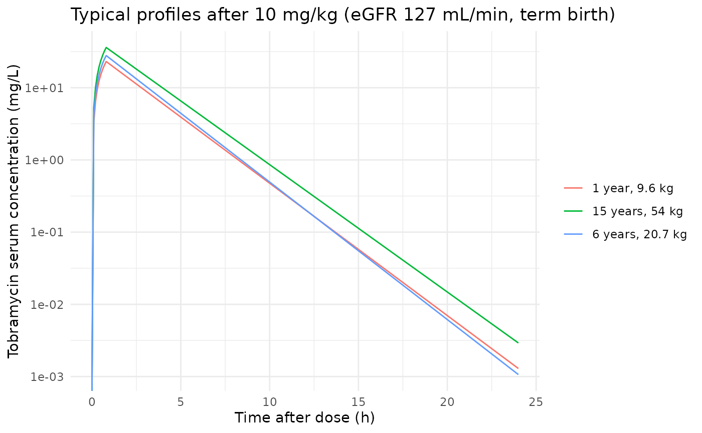
PKNCA validation
AUC over the steady-state dosing interval (48-72 h) is computed with PKNCA per regimen and age group.
sim_nca <- sim |>
  filter(!is.na(Cc)) |>
  select(id, time, Cc, agegrp, regimen)

dose_df <- events |>
  filter(evid == 1) |>
  select(id, time, amt, agegrp, regimen)

conc_obj <- PKNCA::PKNCAconc(sim_nca, Cc ~ time | regimen + agegrp + id)
dose_obj <- PKNCA::PKNCAdose(
  dose_df,
  amt ~ time | regimen + agegrp + id,
  route = "intravascular"
)
intervals <- data.frame(start = 48, end = 72, auclast = TRUE, cmax = TRUE)
nca_res <- PKNCA::pk.nca(PKNCA::PKNCAdata(conc_obj, dose_obj, intervals = intervals))

auc <- as.data.frame(nca_res) |>
  filter(PPTESTCD == "auclast") |>
  select(id, agegrp, regimen, auc = PPORRES) |>
  left_join(
    sim |> distinct(id, cl, dose),
    by = "id"
  ) |>
  mutate(
    auc_closed = dose / cl,
    pct_diff = 100 * (auc - auc_closed) / auc_closed
  )

# Same drawn parameters on both sides (AUC24,ss = Dose / CL at steady state):
# the difference is trapezoidal error plus any residual accumulation only.
stopifnot(
  nrow(auc) == nrow(regimens),
  abs(median(auc$pct_diff)) < 1,
  quantile(abs(auc$pct_diff), 0.9) < 3
)
The PKNCA steady-state AUC agrees with the closed form Dose/CL used by the authors (median difference -0.33%).
Probability of target attainment (Table 4)
pta <- function(d) {
  d |>
    summarise(
      `<80 (%)` = 100 * mean(auc < 80),
      `>110 (%)` = 100 * mean(auc > 110),
      PTA = mean(auc >= 80 & auc <= 110),
      .groups = "drop"
    )
}
pta_sim <- bind_rows(
  auc |> group_by(regimen) |> pta() |> mutate(agegrp = "All ages"),
  auc |> group_by(regimen, agegrp) |> pta() |> mutate(agegrp = as.character(agegrp))
)

published_t4 <- tibble::tribble(
  ~regimen, ~agegrp, ~pub_lt80, ~pub_gt110, ~pub_pta,
  "SOC", "All ages", 49.4, 19.8, 0.31,
  "SOC", "<2 years", 83.3, 1.9, 0.15,
  "SOC", "2-12 years", 60.7, 6.6, 0.33,
  "SOC", ">12 years", 6.7, 57.7, 0.36,
  "Individualized", "All ages", 16.7, 19.3, 0.64,
  "Individualized", "<2 years", 19.1, 19.1, 0.62,
  "Individualized", "2-12 years", 19.8, 17.6, 0.63,
  "Individualized", ">12 years", 13.7, 22.5, 0.64
)

pta_cmp <- published_t4 |>
  left_join(pta_sim |> mutate(regimen = as.character(regimen)), by = c("regimen", "agegrp"))

pta_cmp |>
  transmute(
    Regimen = regimen,
    `Age group` = agegrp,
    `Simulated <80 (%)` = sprintf("%.1f", `<80 (%)`),
    `Published <80 (%)` = pub_lt80,
    `Simulated >110 (%)` = sprintf("%.1f", `>110 (%)`),
    `Published >110 (%)` = pub_gt110,
    `Simulated PTA` = sprintf("%.2f", PTA),
    `Published PTA` = pub_pta
  ) |>
knitr::kable(caption = "Replicates Table 4 of Harwood 2025: target AUC24,ss 80-110 mg*h/L.")| Regimen | Age group | Simulated <80 (%) | Published <80 (%) | Simulated >110 (%) | Published >110 (%) | Simulated PTA | Published PTA |
|---|---|---|---|---|---|---|---|
| SOC | All ages | 49.3 | 49.4 | 17.2 | 19.8 | 0.34 | 0.31 |
| SOC | <2 years | 82.0 | 83.3 | 2.0 | 1.9 | 0.16 | 0.15 |
| SOC | 2-12 years | 56.0 | 60.7 | 9.5 | 6.6 | 0.34 | 0.33 |
| SOC | >12 years | 10.0 | 6.7 | 40.0 | 57.7 | 0.50 | 0.36 |
| Individualized | All ages | 19.0 | 16.7 | 16.0 | 19.3 | 0.65 | 0.64 |
| Individualized | <2 years | 21.5 | 19.1 | 12.5 | 19.1 | 0.66 | 0.62 |
| Individualized | 2-12 years | 15.0 | 19.8 | 20.0 | 17.6 | 0.65 | 0.63 |
| Individualized | >12 years | 20.5 | 13.7 | 15.5 | 22.5 | 0.64 | 0.64 |
ind_all <- pta_cmp |> filter(regimen == "Individualized", agegrp == "All ages")
soc <- pta_cmp |> filter(regimen == "SOC")
stopifnot(
  # Individualized dosing: PTA is set by omega_CL (0.17) and the 80-110 window
  # around the 95 target, so it should sit near the published 0.64.
  abs(ind_all$PTA - 0.64) < 0.08,
  # SOC: under-exposure dominates in <2 years, over-exposure in >12 years.
  soc$`<80 (%)`[soc$agegrp == "<2 years"] > 60,
  soc$`>110 (%)`[soc$agegrp == ">12 years"] > 30
)
AUC24,ss by age group (Figure 1)
ggplot(auc, aes(agegrp, auc, fill = agegrp)) +
  geom_boxplot(outlier.shape = NA, show.legend = FALSE) +
  geom_hline(yintercept = c(80, 110), linetype = "dashed", colour = "red") +
  facet_wrap(~regimen, ncol = 1) +
  coord_cartesian(ylim = c(0, 250)) +
  labs(
    x = NULL,
    y = "AUC24,ss (mg*h/L)",
    title = "Simulated AUC24,ss by age group",
    caption = "Replicates Figure 1 of Harwood 2025."
  ) +
  theme_minimal()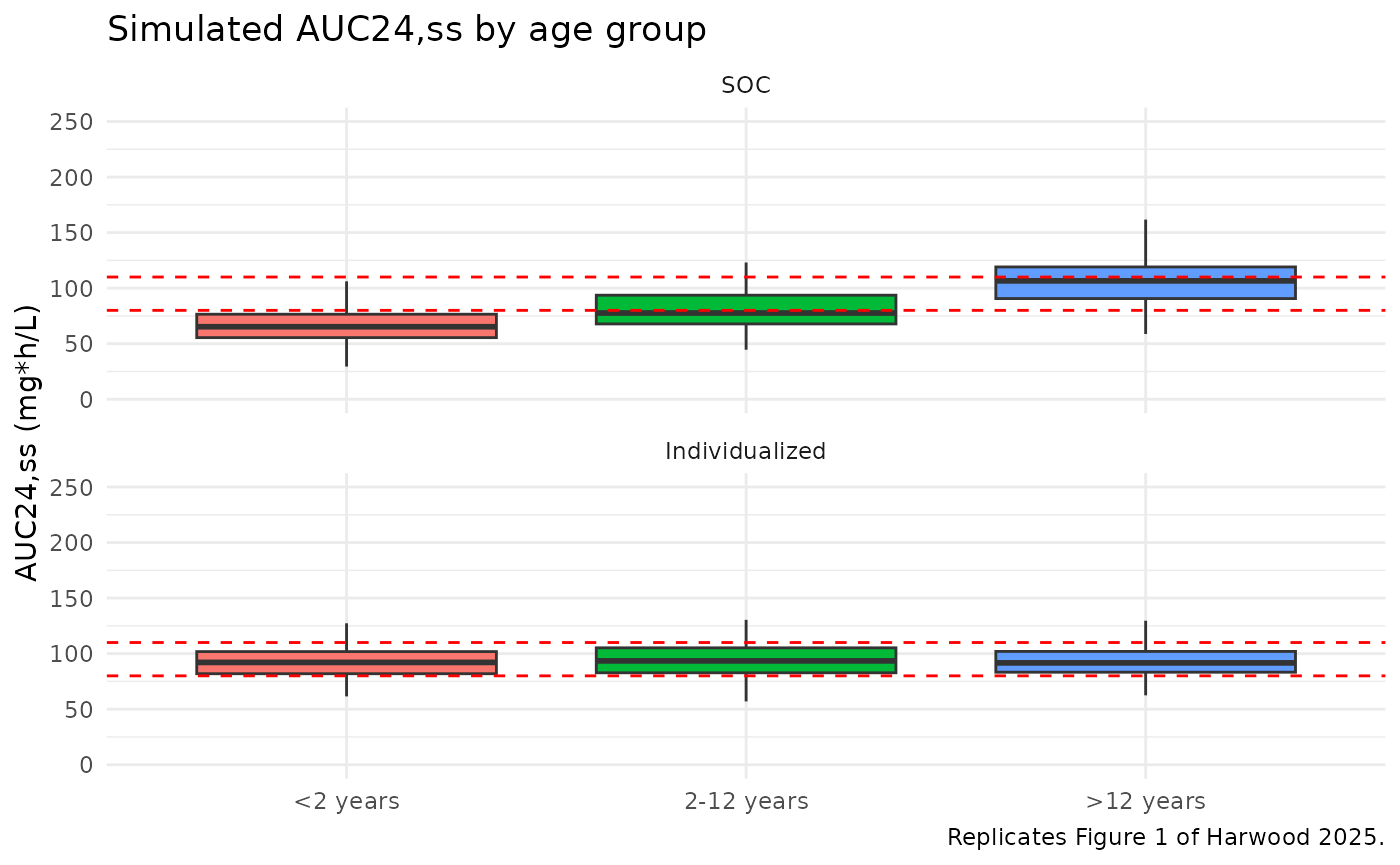
Median AUC24,ss compared with Figure 1
The published medians were read by the maintainers from the box-plot centre lines of Figure 1 (approximately +/- 3 mg*h/L).
published_fig1 <- tibble::tribble(
  ~regimen, ~agegrp, ~auclast,
  "SOC", "<2 years", 63,
  "SOC", "2-12 years", 75,
  "SOC", ">12 years", 115,
  "Individualized", "<2 years", 93,
  "Individualized", "2-12 years", 94,
  "Individualized", ">12 years", 96
)

cmp <- nlmixr2lib::ncaComparisonTable(
  simulated = nca_res,
  reference = published_fig1,
  by = c("regimen", "agegrp"),
  units = c(auclast = "mg*h/L"),
  tolerance_pct = 20
)
knitr::kable(
  cmp,
  caption = "Simulated vs. published median AUC24,ss (48-72 h interval). * differs from reference by >20%."
)| NCA parameter | regimen | agegrp | Reference | Simulated | % diff |
|---|---|---|---|---|---|
| AUClast (mg*h/L) | SOC | <2 years | 63 | 65.3 | +3.6% |
| AUClast (mg*h/L) | SOC | 2-12 years | 75 | 77.6 | +3.5% |
| AUClast (mg*h/L) | SOC | >12 years | 115 | 107 | -7.3% |
| AUClast (mg*h/L) | Individualized | <2 years | 93 | 92.1 | -1.0% |
| AUClast (mg*h/L) | Individualized | 2-12 years | 94 | 93.5 | -0.6% |
| AUClast (mg*h/L) | Individualized | >12 years | 96 | 91.7 | -4.5% |
med <- auc |>
  group_by(regimen, agegrp) |>
  summarise(med = median(auc), .groups = "drop") |>
  mutate(regimen = as.character(regimen), agegrp = as.character(agegrp)) |>
  left_join(published_fig1, by = c("regimen", "agegrp"))
stopifnot(
  # Individualized arm: centred on the 95 mg*h/L target by construction.
  all(abs(med$med[med$regimen == "Individualized"] / 95 - 1) < 0.1),
  # SOC arm: medians within 25% of Figure 1; the covariate database differs.
  all(abs(med$med[med$regimen == "SOC"] / med$auclast[med$regimen == "SOC"] - 1) < 0.25)
)
The individualized-dosing PTA is close to the published 0.62-0.64 in every age group, because once the dose is computed from the typical clearance, attainment depends only on the between-subject variability of clearance and on the dose cap. Standard-of-care PTA and median AUC depend on the joint distribution of weight, height and creatinine in the virtual population, which the paper’s 704-patient covariate database determines and this vignette only approximates; the qualitative pattern (marked under-exposure in children under 2 years and over-exposure in adolescents) is reproduced. The largest difference is the share of adolescents above 110 mg*h/L with standard dosing, which is the stratum most sensitive to the assumed eGFR distribution: at a fixed mg/kg dose, AUC scales with eGFR^-0.4, so an adolescent covariate database with a lower median eGFR than the Table 1 value used here moves more of that group above the window.
Assumptions and deviations
- Virtual covariates. The authors’ 704-patient covariate database is not public. Weight and height are drawn around approximate growth-chart medians for age chosen by the maintainers, and eGFR around the Table 1 median of 127 mL/min with a 25% log-scale SD truncated to the Table 1 range; serum creatinine is back-calculated from the modified Schwartz equation. These choices affect only the standard-of-care comparison.
- Residual-error scale. Table 3 labels the between-subject variability rows as standard deviations but does not say whether the additive (0.173) and proportional (0.103) residual-error estimates are SDs or variances. They are encoded as SDs (0.173 mg/L and 10.3%), the usual reporting for a combined error model; as variances they would imply a 32% proportional error, which is implausible for an immunoassay. Residual error does not enter any check here.
- Between-subject variability. Table 3 reports omega as a standard deviation; variances are entered as SD^2. The individualized-dosing PTA of about 0.64 that the authors report is what a log-normal CL with SD 0.17 gives for an 80-110 window around a target of 95, which supports this reading.
-
Gestational age. The model takes
GAso that postmenstrual age isAGE * 52 + GA. The authors assumed 40 weeks when gestational age was not recorded, and the published dosing equation hard-codes 40; all simulations here useGA = 40. -
Units. Height enters as the canonical
HTin cm and is divided by 100 inside the model; creatinine enters asCREATin mg/dL as in Supplementary Eq. 5 (Table 1 reports umol/L; divide by 88.4). - eGFR centring. The equations centre eGFR on 127.3 mL/min while Table 1 reports a median of 127; the equation value is used.
-
Infusion duration. D1 is the fitted duration of the
zero-order input (0.801 h, against a documented 0.5 h infusion). Dose
records must carry
rate = -2for the model to use it. The Table 3 footnote calls D1 a “rate of infusion”, but the Results text and Supplementary Eq. 3 define it as a duration in hours. - No erratum or correction notice was found for this article as of 2026-11-05.