Vancomycin (Zhou 2019)

Model and source

• Citation: Zhou Y, Gao F, Chen C, Ma L, Yang T, Liu X, Liu Y, Wang X, Zhao X, Que C, Li S, Lv J, Cui Y, Yang L. Development of a Population Pharmacokinetic Model of Vancomycin and its Application in Chinese Geriatric Patients with Pulmonary Infections. Eur J Drug Metab Pharmacokinet. 2019;44(3):361-370. doi:10.1007/s13318-018-0534-2
• Description: One-compartment IV population PK model for vancomycin in 70 Chinese geriatric patients (age >= 65 years) with hospital- or community-acquired pulmonary infection (Zhou 2019). Clearance scales by power exponent with raw Cockcroft-Gault creatinine clearance (mL/min, reference 56.28); volume of distribution carries no retained covariate. Estimated from 125 steady-state trough concentrations collected by routine therapeutic drug monitoring.
• Article: https://doi.org/10.1007/s13318-018-0534-2 (open access, CC BY-NC 4.0)

Population

Zhou 2019 is a retrospective, single-centre therapeutic-drug-monitoring (TDM) study at Peking University First Hospital. Seventy Chinese inpatients aged 65 years or older, treated with intravenous vancomycin for at least two days for hospital-acquired (57 patients, 81.4%) or community-acquired (13 patients, 18.6%) pneumonia, contributed 125 vancomycin concentrations (1-5 per patient, mean 1.79). Baseline characteristics are in the paper’s Table 1: 49 male / 21 female, age 78.3 +/- 6.96 years, weight 60.7 +/- 10.2 kg, height 161 +/- 10 cm, Cockcroft-Gault creatinine clearance 56.3 +/- 22.1 mL/min, serum creatinine 90.6 +/- 31 umol/L, mean daily dose 1.55 +/- 0.770 g/day and observed concentration 17 +/- 8.03 mg/L. Patients with multiple organ failure, renal replacement therapy or low-volume shock were excluded.

The single most important feature of this dataset for anyone reusing the model is that every observation is a trough. Section 3.2 states that TDM samples were drawn 0.5-2 h before and after the fourth or fifth dose and that the pre-dose values “were regarded as steady-state concentrations”; Section 3.3 confirms “the serum concentrations in the study were trough concentrations in steady-state”. With no peak or distribution-phase samples, the volume of distribution is only weakly identified by the data, and the reported 154 L (about 2.5 L/kg at the cohort mean weight, against a textbook vancomycin value near 0.7 L/kg) is correspondingly high. Combined with CL = 2.45 L/h it implies a typical terminal half-life of about 44 h. This is a property of the published model, not a transcription error, and it is reproduced faithfully here; the “Assumptions and deviations” section returns to it.

The same information is available programmatically via the model’s population metadata (readModelDb("Zhou_2019_vancomycin")()$population).

Source trace

The per-parameter origin is recorded as an in-file comment next to each ini() entry in inst/modeldb/specificDrugs/Zhou_2019_vancomycin.R. The table below collects them in one place for review.

Equation / parameter	Value	Source location
lcl (CL at CLCR = 56.28 mL/min)	log(2.45) L/h	Table 3, row theta_1CL, “Final model” column (RSE 6.9%); bootstrap median 2.43, 95% CI (2.09, 2.81) in Table 4
lvc (volume of distribution)	log(154) L	Table 3, row theta_2Vd (RSE 9.2%); bootstrap median 154, 95% CI (117, 191) in Table 4
e_crcl_cl (power exponent on CLCR)	0.542	Table 3, row theta_3CLCR (mL/min) on CL (RSE 35.1%); bootstrap median 0.538, 95% CI (0.206, 0.878) in Table 4; also the exponent in Eq. (9)
etalcl (IIV variance on CL)	0.174	Table 3, row omega CL (RSE 21.2%); bootstrap median 0.162, 95% CI (0.092, 0.256) in Table 4
etalvc (IIV variance on Vd)	0.339	Table 3, row omega V (RSE 37.8%); bootstrap median 0.289, 95% CI (0.121, 0.557) in Table 4
propSd (proportional residual SD)	0.2563 = sqrt(0.0657)	Table 3, row sigma_1 = 0.0657 (RSE 34.2%), a NONMEM $SIGMA variance
addSd (additive residual SD)	fixed(0)	Table 3, row sigma_2 = “0 FIX”
CL covariate model	cl <- exp(lcl + etalcl) * (CRCL/56.28)^e_crcl_cl	Eq. (9): CL (L/h) = 2.45 * (CLCR/56.28)^0.542, combined with the exponential IIV of Eq. (1) and the power covariate form of Eq. (6)
Vd covariate model	vc <- exp(lvc + etalvc)	Eq. (10): Vd (L) = 154 (no retained covariate), with the exponential IIV of Eq. (2)
Structure (one compartment, first-order elimination)	n/a	Section 3.3: “we established a one-compartment model that with first-order elimination (ADVAN1 TRANS2)”
Residual error (combined, additive term zero)	n/a	Eq. (3): C_i,obs = C_i,pre * (1 + eps1) + eps2
Reference CLCR 56.28 mL/min	56.28	Eq. (9) denominator; equals the Table 1 cohort mean 56.3 mL/min to four significant figures

Two transcription hazards in this paper

Both were resolved from the paper itself and are recorded here because a reader checking this extraction against the PDF will hit them.

1. The abstract drops the exponent. The Abstract Results renders Eq. (9) as “clearance (CL) [L/h] = 2.45 x (CL CR /56.28) x 0.542” – the superscript 0.542 has been flattened into a multiplication. The Discussion (Section 5) prints the same equation correctly as CL(L/h) = 2.45 x (CLCR/56.28)^0.542, Table 3 labels the value “theta_3CLCR (mL/min) on CL” (a covariate coefficient, not a scale factor), and Eq. (6) gives the retained functional form as CL_i = TV(CL) x (covariate/typical value)^theta. The power form is used here. Reading it as a multiplication would also be internally absurd: it would make the typical CL 2.45 x 1 x 0.542 = 1.33 L/h rather than the 2.45 L/h that Table 3 and the Abstract both state.
2. “Eq. (3)” in Section 4 is a mis-citation. Section 4 says “When the influences of continuous covariates were validated by Eq. (3), the OFV was satisfied better”, but Eq. (3) is the residual-error model. The covariate forms are Eqs. (4)-(6); Eq. (6) is the power model that Eq. (9) instantiates. Following the standing policy of trusting the printed equation over the prose, Eq. (6)/(9) is authoritative.

Virtual cohort

Original observed data are not publicly available. The cohort below draws creatinine clearance from the Table 1 summary (mean 56.3 mL/min, SD 22.1), truncated to a physiologically possible 10-130 mL/min, and simulates the seven dosing regimens the paper itself simulated in its Table 5.

# `set.seed()` seeds R's RNG. It does NOT seed rxode2's simulation RNG, and
# rxode2's streams are partitioned PER SOLVER THREAD -- so this cohort is
# reproducible on this machine and different on a machine with a different
# thread count. Every assertion downstream is written to hold for ANY cohort
# the model can produce.
set.seed(20190330)

n_per_arm <- 200L # cap is 200 per arm

# Section 3.2: "500 mg (every 6 h, 8 h, 12 h, 24 h, 48 h) and 1000 mg (every
# 8 h, 12 h), for 1.5-2 h intravenous infusion". Table 5 simulates these seven
# regimens.
regimens <- tibble::tribble(
  ~regimen,          ~amt,  ~tau,
  "1000 mg q8h",     1000,  8,
  "1000 mg q12h",    1000, 12,
  "1000 mg q24h",    1000, 24,
  "500 mg q6h",       500,  6,
  "500 mg q8h",       500,  8,
  "500 mg q12h",      500, 12,
  "500 mg q24h",      500, 24
)

# Infusion duration: the paper gives a 1.5-2 h range and never a single value.
# The midpoint is used; the sensitivity chunk below shows the trough is
# insensitive to the choice across the whole stated range.
t_inf <- 1.75

# Cockcroft-Gault CLCR, Table 1: mean 56.3, SD 22.1 mL/min. Rejection-sample
# into [10, 130] so no subject gets a non-physiological renal function. This
# raises the realised mean about 1 mL/min above 56.3.
draw_crcl <- function(n) {
  out <- numeric(0)
  while (length(out) < n) {
    x <- stats::rnorm(2L * n, mean = 56.3, sd = 22.1)
    out <- c(out, x[x >= 10 & x <= 130])
  }
  out[seq_len(n)]
}

make_arm <- function(regimen, amt, tau, id_offset) {
  subj <- tibble::tibble(
    id = id_offset + seq_len(n_per_arm),
    CRCL = draw_crcl(n_per_arm),
    regimen = regimen
  )
  # Four doses at 0, tau, 2*tau, 3*tau -- Section 3.2 samples TDM "before the
  # fourth or fifth dose", and the trough before the fifth dose is the quantity
  # Table 5 reports (see the validation section).
  dosing <- subj |>
    tidyr::crossing(dose_no = 0:3) |>
    dplyr::mutate(
      time = dose_no * tau, amt = amt, evid = 1L, dur = t_inf,
      cmt = "central"
    ) |>
    dplyr::select(-dose_no)
  # Observations: a profile grid over the whole 0-4*tau window for the figure,
  # plus exact records at 3*tau and 4*tau so PKNCA can anchor the fourth
  # dosing interval and return Ctrough at its end.
  # Rounding collapses floating-point near-duplicates: seq() renders 3*tau as
  # 24.000000000000004 for tau = 8, which would otherwise survive distinct()
  # alongside the exact 24 and put two almost-identical records in the PKNCA
  # input. The interval bounds 3*tau and 4*tau must be EXACT, because PKNCA
  # matches Ctrough and Cstart with `time %in% end` / `%in% start`.
  obs_times <- unique(round(
    c(seq(0, 4 * tau, length.out = 161L), 3 * tau, 4 * tau),
    9
  ))
  obs <- subj |>
    tidyr::crossing(time = obs_times) |>
    dplyr::mutate(amt = NA_real_, evid = 0L, dur = NA_real_, cmt = "central")
  dplyr::bind_rows(dosing, obs) |>
    dplyr::distinct(id, time, evid, .keep_all = TRUE) |>
    dplyr::arrange(id, time, dplyr::desc(evid))
}

events <- do.call(
  dplyr::bind_rows,
  lapply(seq_len(nrow(regimens)), function(i) {
    make_arm(
      regimens$regimen[i], regimens$amt[i], regimens$tau[i],
      id_offset = (i - 1L) * n_per_arm
    )
  })
)

# Disjoint IDs across arms: duplicate IDs are silently merged by rxSolve into a
# single subject receiving the summed dose.
stopifnot(!anyDuplicated(unique(events[, c("id", "time", "evid")])))
stopifnot(dplyr::n_distinct(events$id) == n_per_arm * nrow(regimens))

Simulation

mod <- readModelDb("Zhou_2019_vancomycin")

sim <- rxode2::rxSolve(
  mod,
  events = events,
  keep = c("regimen", "CRCL"),
  # The model is written as an explicit ODE; keep it that way rather than
  # letting rxSolve's ODE -> linCmt auto-conversion decide.
  useLinCmt = FALSE
) |>
  as.data.frame()
#> ℹ parameter labels from comments will be replaced by 'label()'

if (is.null(sim$id)) sim$id <- 1L
stopifnot(nrow(sim) > 0L, !all(is.na(sim$Cc)))

Replicate published figures

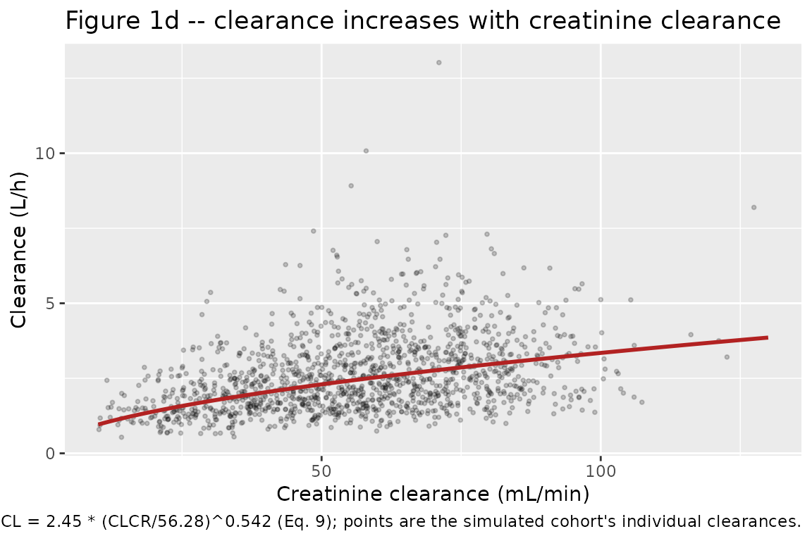
Figure 1d – clearance versus creatinine clearance

Figure 1 of Zhou 2019 plots base-model individual clearances against each continuous covariate; panel (d) shows CL rising with CLCR, the relationship Eq. (9) formalises. The line below is the typical-value relationship and the points are the simulated cohort’s individual clearances.

# Replicates Figure 1d of Zhou 2019: CL versus CLCR.
cl_typical <- tibble::tibble(CRCL = seq(10, 130, by = 1)) |>
  dplyr::mutate(cl = 2.45 * (CRCL / 56.28)^0.542)

sim |>
  dplyr::distinct(id, CRCL, cl) |>
  ggplot(aes(CRCL, cl)) +
  geom_point(alpha = 0.2, size = 0.7) +
  geom_line(data = cl_typical, colour = "firebrick", linewidth = 1) +
  labs(
    x = "Creatinine clearance (mL/min)", y = "Clearance (L/h)",
    title = "Figure 1d -- clearance increases with creatinine clearance",
    caption = paste(
      "Replicates Figure 1d of Zhou 2019. Red line is the typical-value",
      "relationship CL = 2.45 * (CLCR/56.28)^0.542 (Eq. 9); points are the",
      "simulated cohort's individual clearances."
    )
  )

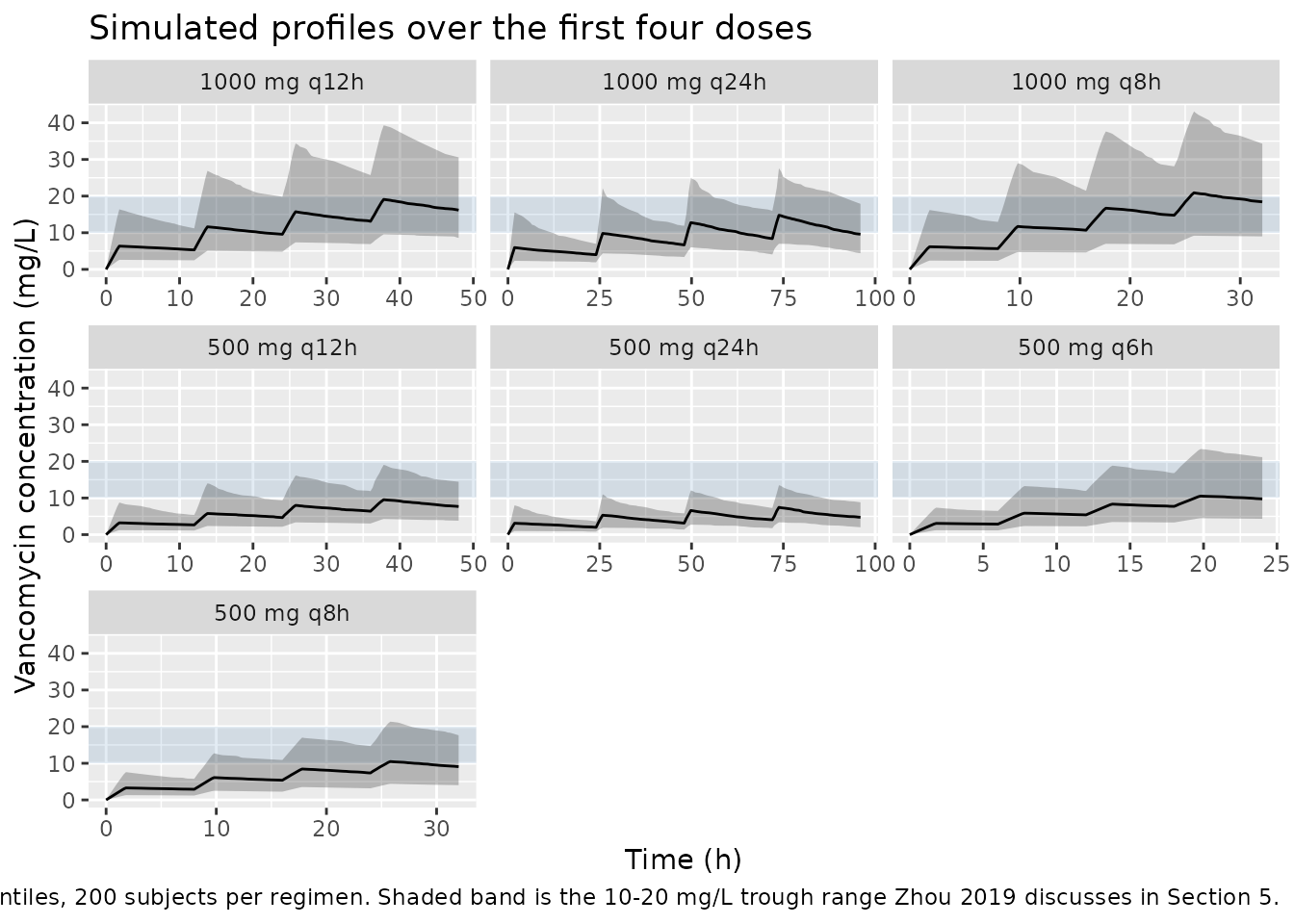
Concentration-time profiles for the Table 5 regimens

sim |>
  dplyr::group_by(regimen, time) |>
  dplyr::summarise(
    Q05 = quantile(Cc, 0.05, na.rm = TRUE),
    Q50 = quantile(Cc, 0.50, na.rm = TRUE),
    Q95 = quantile(Cc, 0.95, na.rm = TRUE),
    .groups = "drop"
  ) |>
  ggplot(aes(time, Q50)) +
  annotate(
    "rect",
    xmin = -Inf, xmax = Inf, ymin = 10, ymax = 20,
    alpha = 0.15, fill = "steelblue"
  ) +
  geom_ribbon(aes(ymin = Q05, ymax = Q95), alpha = 0.3) +
  geom_line() +
  facet_wrap(~regimen, scales = "free_x") +
  labs(
    x = "Time (h)", y = "Vancomycin concentration (mg/L)",
    title = "Simulated profiles over the first four doses",
    caption = paste(
      "Median and 5th-95th percentiles, 200 subjects per regimen. Shaded band",
      "is the 10-20 mg/L trough range Zhou 2019 discusses in Section 5."
    )
  )

Deterministic structural checks

These compare the packaged model against closed-form algebra for a typical subject with the random effects zeroed. Both sides use the same parameters, so the only difference is numerical, and the tolerances are correspondingly tight.

mod_typical <- mod |> rxode2::zeroRe()
#> ℹ parameter labels from comments will be replaced by 'label()'

# Closed-form trough at t = n*tau for n equal-interval infusions of duration
# t_inf into a one-compartment model, by superposition.
trough_closed_form <- function(amt, tau, n_dose, cl, vc, t_inf) {
  k <- cl / vc
  t_end <- n_dose * tau
  sum(vapply(
    seq_len(n_dose) - 1L,
    function(j) {
      (amt / (t_inf * cl)) * (1 - exp(-k * t_inf)) *
        exp(-k * (t_end - (j * tau + t_inf)))
    },
    numeric(1)
  ))
}

crcl_ref <- 56.28
cl_ref <- 2.45 * (crcl_ref / 56.28)^0.542
vc_ref <- 154

gate_cf <- regimens |>
  dplyr::rowwise() |>
  dplyr::mutate(
    closed_form = trough_closed_form(amt, tau, 4L, cl_ref, vc_ref, t_inf),
    solved = {
      ev <- rxode2::et(
        amt = amt, dur = t_inf, ii = tau, until = 3 * tau, cmt = "central"
      ) |>
        rxode2::et(time = 4 * tau, cmt = "central")
      ev <- as.data.frame(ev)
      ev$CRCL <- crcl_ref
      s <- rxode2::rxSolve(
        mod_typical, ev,
        returnType = "data.frame", useLinCmt = FALSE
      )
      s$Cc[abs(s$time - 4 * tau) < 1e-8][1]
    }
  ) |>
  dplyr::ungroup() |>
  dplyr::mutate(pct_diff = 100 * (solved - closed_form) / closed_form)
#> ℹ omega/sigma items treated as zero: 'etalcl', 'etalvc'
#> ℹ omega/sigma items treated as zero: 'etalcl', 'etalvc'
#> ℹ omega/sigma items treated as zero: 'etalcl', 'etalvc'
#> ℹ omega/sigma items treated as zero: 'etalcl', 'etalvc'
#> ℹ omega/sigma items treated as zero: 'etalcl', 'etalvc'
#> ℹ omega/sigma items treated as zero: 'etalcl', 'etalvc'
#> ℹ omega/sigma items treated as zero: 'etalcl', 'etalvc'

gate_cf |>
  dplyr::select(regimen, closed_form, solved, pct_diff) |>
  dplyr::rename(
    "Regimen" = regimen,
    "Closed form (mg/L)" = closed_form,
    "rxode2 solve (mg/L)" = solved,
    "% diff" = pct_diff
  ) |>
  knitr::kable(
    digits = 4,
    caption = paste(
      "Trough before the fifth dose: rxode2 solve of the packaged model versus",
      "closed-form superposition, typical subject (CLCR = 56.28 mL/min)."
    )
  )

Trough before the fifth dose: rxode2 solve of the packaged model versus closed-form superposition, typical subject (CLCR = 56.28 mL/min).

Regimen	Closed form (mg/L)	rxode2 solve (mg/L)	% diff
1000 mg q8h	19.3553	19.3554	3e-04
1000 mg q12h	16.7172	16.7173	3e-04
1000 mg q24h	11.0874	11.0874	3e-04
500 mg q6h	10.4328	10.4328	-1e-04
500 mg q8h	9.6777	9.6777	3e-04
500 mg q12h	8.3586	8.3586	3e-04
500 mg q24h	5.5437	5.5437	3e-04

# Deterministic: pure numerical error between two evaluations of the same
# algebra. This also proves the event table's `dur =` is honoured -- if the
# infusion were silently delivered as a bolus these would diverge.
stopifnot(nrow(gate_cf) == 7L, !anyNA(gate_cf$solved))
stopifnot(max(abs(gate_cf$pct_diff)) < 0.1)

# Eq. (9) exactly: cl from the model must equal 2.45 * (CLCR/56.28)^0.542.
crcl_grid <- c(15, 30, 50, 56.28, 75, 100, 125)
ev_cl <- data.frame(
  id = seq_along(crcl_grid),
  time = 0, amt = 1000, evid = 1L, dur = t_inf, cmt = "central",
  CRCL = crcl_grid
)
ev_cl <- dplyr::bind_rows(
  ev_cl,
  transform(ev_cl, time = 1, amt = NA_real_, evid = 0L, dur = NA_real_)
)
cl_check <- rxode2::rxSolve(
  mod_typical, ev_cl,
  keep = "CRCL", returnType = "data.frame", useLinCmt = FALSE
) |>
  dplyr::distinct(id, CRCL, cl, vc) |>
  dplyr::mutate(
    cl_eq9 = 2.45 * (CRCL / 56.28)^0.542,
    cl_rel = abs(cl - cl_eq9) / cl_eq9,
    vc_rel = abs(vc - 154) / 154
  )
#> ℹ omega/sigma items treated as zero: 'etalcl', 'etalvc'
#> Warning: multi-subject simulation without without 'omega'

stopifnot(nrow(cl_check) == length(crcl_grid))
stopifnot(max(cl_check$cl_rel) < 1e-8, max(cl_check$vc_rel) < 1e-8)

cl_check |>
  dplyr::select(CRCL, cl, cl_eq9) |>
  dplyr::rename(
    "CLCR (mL/min)" = CRCL,
    "Model CL (L/h)" = cl,
    "Eq. (9) CL (L/h)" = cl_eq9
  ) |>
  knitr::kable(
    digits = 4,
    caption = "Model clearance reproduces Eq. (9) exactly across the CLCR range."
  )

Model clearance reproduces Eq. (9) exactly across the CLCR range.

CLCR (mL/min)	Model CL (L/h)	Eq. (9) CL (L/h)
15.00	1.1965	1.1965
30.00	1.7421	1.7421
50.00	2.2978	2.2978
56.28	2.4500	2.4500
75.00	2.8626	2.8626
100.00	3.3456	3.3456
125.00	3.7757	3.7757

# Lower renal function must give a HIGHER trough. This is a deterministic
# comparison (random effects zeroed), so asserting the direction is safe --
# it would not be on a simulated cohort.
direction <- regimens |>
  dplyr::rowwise() |>
  dplyr::mutate(
    trough_crcl30 = trough_closed_form(
      amt, tau, 4L, 2.45 * (30 / 56.28)^0.542, vc_ref, t_inf
    ),
    trough_crcl90 = trough_closed_form(
      amt, tau, 4L, 2.45 * (90 / 56.28)^0.542, vc_ref, t_inf
    )
  ) |>
  dplyr::ungroup()

stopifnot(all(direction$trough_crcl30 > direction$trough_crcl90))

PKNCA validation

PKNCA is run over the fourth dosing interval, whose end-point concentration is the trough before the fifth dose – the quantity the paper’s Table 5 reports (see the next section for why).

The interval is presented to PKNCA with its time origin at the fourth dose rather than in absolute time. This is required, not cosmetic: PKNCA::pk.calc.ctrough() selects the end-point concentration with time %in% end, but pk.nca() re-bases each interval’s concentration times onto the most recent dose while still passing end in absolute time. For an interval [3*tau, 4*tau] the two frames disagree and every ctrough comes back NA. Rebasing so the fourth dose sits at time 0 and the interval is [0, tau] makes the two frames agree. (ctau is not an accepted interval column in the installed PKNCA, so it is not an alternative here.)

tau_lookup <- stats::setNames(regimens$tau, regimens$regimen)

# Restrict to the fourth dosing interval and move its origin to zero.
sim_nca <- sim |>
  dplyr::filter(!is.na(Cc)) |>
  dplyr::mutate(tau = tau_lookup[regimen]) |>
  dplyr::filter(time >= 3 * tau, time <= 4 * tau) |>
  dplyr::mutate(time_rel = round(time - 3 * tau, 9)) |>
  dplyr::select(id, time_rel, Cc, regimen, tau)

stopifnot(nrow(sim_nca) > 0L)
# The interval bounds must be present EXACTLY for Ctrough / Cstart to resolve.
stopifnot(
  all(tapply(sim_nca$time_rel, sim_nca$id, function(z) 0 %in% z)),
  all(
    mapply(
      function(z, tt) tt %in% z,
      split(sim_nca$time_rel, sim_nca$id),
      tapply(sim_nca$tau, sim_nca$id, dplyr::first)
    )
  )
)

conc_obj <- PKNCA::PKNCAconc(
  as.data.frame(sim_nca), Cc ~ time_rel | regimen + id
)

# One dose per subject, at the rebased origin of the interval.
dose_df <- sim_nca |>
  dplyr::distinct(id, regimen) |>
  dplyr::left_join(regimens, by = "regimen") |>
  dplyr::transmute(id, regimen, time_rel = 0, amt) |>
  as.data.frame()

dose_obj <- PKNCA::PKNCAdose(dose_df, amt ~ time_rel | regimen + id)

# One interval per regimen: the whole (rebased) fourth dosing interval.
intervals <- regimens |>
  dplyr::transmute(
    regimen,
    start = 0,
    end = tau,
    ctrough = TRUE,
    cstart = TRUE,
    cmax = TRUE,
    tmax = TRUE,
    cav = TRUE,
    auclast = TRUE
  ) |>
  as.data.frame()

nca_res <- PKNCA::pk.nca(
  PKNCA::PKNCAdata(conc_obj, dose_obj, intervals = intervals)
)

nca_wide <- as.data.frame(nca_res) |>
  dplyr::filter(
    PPTESTCD %in% c("ctrough", "cstart", "cmax", "tmax", "cav", "auclast")
  ) |>
  dplyr::select(regimen, id, PPTESTCD, PPORRES) |>
  tidyr::pivot_wider(names_from = PPTESTCD, values_from = PPORRES)

# A gate that cannot go red is worse than none: confirm every subject is
# present AND that Ctrough actually resolved for each of them.
stopifnot(nrow(nca_wide) == n_per_arm * nrow(regimens))
stopifnot(!anyNA(nca_wide$ctrough), !anyNA(nca_wide$cstart))

# Still accumulating at the fourth dose, so the interval-end trough must exceed
# the interval-start trough for every subject. This is a structural consequence
# of the 44 h half-life against a <= 24 h dosing interval, not a noise-sensitive
# comparison.
stopifnot(all(nca_wide$ctrough > nca_wide$cstart))

Steady-state dose recovery

At steady state the area under one dosing interval must equal Dose / CL exactly, whatever the infusion duration. This is run on a typical subject with a long loading period (the typical half-life is about 44 h, so 600 h is more than thirteen half-lives) and a fine grid, so the residual difference is trapezoidal error alone.

ss_one <- function(amt, tau, cl, vc) {
  t0 <- 600
  ev <- rxode2::et(
    amt = amt, dur = t_inf, ii = tau,
    until = t0 + tau, cmt = "central"
  ) |>
    rxode2::et(time = seq(t0, t0 + tau, by = 0.02), cmt = "central")
  ev <- as.data.frame(ev)
  ev$CRCL <- crcl_ref
  s <- rxode2::rxSolve(
    mod_typical, ev,
    returnType = "data.frame", useLinCmt = FALSE
  )
  s <- s[s$time >= t0 & s$time <= t0 + tau, ]
  auc <- PKNCA::pk.calc.auc(
    conc = s$Cc, time = s$time,
    interval = c(t0, t0 + tau), method = "linear", auc.type = "AUClast"
  )
  c(auc = auc, recovery = cl * auc / amt)
}

recovery <- regimens |>
  dplyr::rowwise() |>
  dplyr::mutate(
    auc_tau = ss_one(amt, tau, cl_ref, vc_ref)[["auc"]],
    recovery = ss_one(amt, tau, cl_ref, vc_ref)[["recovery"]]
  ) |>
  dplyr::ungroup()
#> ℹ omega/sigma items treated as zero: 'etalcl', 'etalvc'
#> ℹ omega/sigma items treated as zero: 'etalcl', 'etalvc'
#> ℹ omega/sigma items treated as zero: 'etalcl', 'etalvc'
#> ℹ omega/sigma items treated as zero: 'etalcl', 'etalvc'
#> ℹ omega/sigma items treated as zero: 'etalcl', 'etalvc'
#> ℹ omega/sigma items treated as zero: 'etalcl', 'etalvc'
#> ℹ omega/sigma items treated as zero: 'etalcl', 'etalvc'
#> ℹ omega/sigma items treated as zero: 'etalcl', 'etalvc'
#> ℹ omega/sigma items treated as zero: 'etalcl', 'etalvc'
#> ℹ omega/sigma items treated as zero: 'etalcl', 'etalvc'
#> ℹ omega/sigma items treated as zero: 'etalcl', 'etalvc'
#> ℹ omega/sigma items treated as zero: 'etalcl', 'etalvc'
#> ℹ omega/sigma items treated as zero: 'etalcl', 'etalvc'
#> ℹ omega/sigma items treated as zero: 'etalcl', 'etalvc'

recovery |>
  dplyr::select(regimen, auc_tau, recovery) |>
  dplyr::rename(
    "Regimen" = regimen,
    "AUCtau (mg*h/L)" = auc_tau,
    "CL * AUCtau / Dose" = recovery
  ) |>
  knitr::kable(
    digits = 4,
    caption = paste(
      "Steady-state mass balance: clearance times AUC over one dosing interval",
      "recovers the administered dose."
    )
  )

Steady-state mass balance: clearance times AUC over one dosing interval recovers the administered dose.

Regimen	AUCtau (mg*h/L)	CL * AUCtau / Dose
1000 mg q8h	408.1365	0.9999
1000 mg q12h	408.1385	0.9999
1000 mg q24h	408.1429	1.0000
500 mg q6h	204.0678	0.9999
500 mg q8h	204.0683	0.9999
500 mg q12h	204.0693	0.9999
500 mg q24h	204.0715	1.0000

# Deterministic; the only error source is linear-trapezoidal integration on a
# 0.02 h grid.
stopifnot(nrow(recovery) == 7L, !anyNA(recovery$recovery))
stopifnot(max(abs(recovery$recovery - 1)) < 0.005)

Comparison against the published simulation (Table 5)

Zhou 2019 has no NCA table – it reports no Cmax, Tmax, AUC or half-life. What it does report, in Table 5, is the mean +/- SD concentration from a 1000-run simulation of each of the seven regimens. Two things have to be established before those numbers can be used as a validation target.

Which concentration is it? Table 5’s column header says “Total (average plasma concentration)”, but the values cannot be interval-average concentrations: at steady state Cavg = Dose/(tau * CL), which for 1000 mg q8h is 3000 / (24 * 2.45) = 51 mg/L, not the 19.26 mg/L printed. Nor are they steady-state troughs, which for the same regimen are about 48 mg/L (the 44 h half-life makes accumulation over q8h dosing large). They are the trough before the fifth dose – exactly where Section 3.2 says the TDM samples were drawn (“0.5-2 h before … the fourth or fifth dose”). Computing that quantity reproduces all seven values, whereas the trough before the fourth dose is uniformly 15-20% high. Section 5 confirms the intent: the values are discussed against the 10-20 mg/L trough target, not against an average concentration.

On what scale are the omegas? Table 3 prints omega CL = 0.174 and omega V = 0.339 without stating whether they are variances or standard deviations. Table 5 settles it, because it prints SDs alongside the means: the published between-subject coefficients of variation are 45.6-52.1% across the seven regimens. Reading the omegas as NONMEM $OMEGA variances reproduces that spread: the simulated Cc trough gives 41-48% (table below), and adding the proportional residual term in quadrature – which the paper’s $SIMULATION would have drawn, and Cc excludes – gives 48-55%, bracketing the published range. Reading the same numbers as standard deviations gives only about 22%, half the published value. The variance reading is used, which is also the NONMEM convention the FOCE-I / $OMEGA provenance implies.

# Zhou 2019 Table 5, transcribed. "Total" is the all-subject column; the two
# strata are split at CLCR = 50 mL/min.
table5 <- tibble::tribble(
  ~regimen,       ~total_mean, ~total_sd, ~hi_mean, ~hi_sd, ~lo_mean, ~lo_sd,
  "1000 mg q8h",        19.26,      9.50,    18.41,   8.95,    20.72,   9.53,
  "1000 mg q12h",       16.02,      7.51,    15.10,   7.02,    17.63,   8.44,
  "1000 mg q24h",       10.29,      4.69,     9.40,   4.38,    11.96,   5.30,
  "500 mg q6h",         11.22,      5.85,    10.83,   4.57,    11.88,   4.36,
  "500 mg q8h",          9.82,      4.97,     9.38,   3.65,    10.57,   3.57,
  "500 mg q12h",         7.98,      3.94,     7.52,   2.68,     8.79,   3.43,
  "500 mg q24h",         5.06,      2.53,     4.62,   1.35,     5.89,   2.90
)

# Table 5 reports MEANS, so the simulated side is pre-aggregated to means.
# (ncaComparisonTable() would otherwise aggregate with median(), which for a
# ~50% CV distribution sits about 11% below the mean -- a systematic bias
# against a table of means.)
simulated_mean <- nca_wide |>
  dplyr::group_by(regimen) |>
  dplyr::summarise(ctrough = mean(ctrough), .groups = "drop") |>
  as.data.frame()

published <- table5 |>
  dplyr::transmute(regimen, ctrough = total_mean) |>
  as.data.frame()

cmp <- nlmixr2lib::ncaComparisonTable(
  simulated = simulated_mean,
  reference = published,
  by = "regimen",
  units = c(ctrough = "mg/L"),
  tolerance_pct = 20
)

knitr::kable(
  cmp,
  caption = paste(
    "Trough before the fifth dose: simulated cohort mean versus Zhou 2019",
    "Table 5 'Total' column. * differs from reference by >20%."
  ),
  align = c("l", "l", "r", "r", "r")
)

Trough before the fifth dose: simulated cohort mean versus Zhou 2019 Table 5 ‘Total’ column. * differs from reference by >20%.

NCA parameter	regimen	Reference	Simulated	% diff
Ctrough (mg/L)	1000 mg q8h	19.3	19.5	+1.1%
Ctrough (mg/L)	1000 mg q12h	16	17.1	+7.0%
Ctrough (mg/L)	1000 mg q24h	10.3	10.2	-1.0%
Ctrough (mg/L)	500 mg q6h	11.2	10.8	-4.0%
Ctrough (mg/L)	500 mg q8h	9.82	10	+2.1%
Ctrough (mg/L)	500 mg q12h	7.98	8.06	+1.0%
Ctrough (mg/L)	500 mg q24h	5.06	5.02	-0.8%

attr(cmp, "footnote")
#> NULL

gate_t5 <- simulated_mean |>
  dplyr::left_join(published, by = "regimen", suffix = c("_sim", "_pub")) |>
  dplyr::mutate(pct_diff = 100 * (ctrough_sim - ctrough_pub) / ctrough_pub)

stopifnot(nrow(gate_t5) == 7L, !anyNA(gate_t5$pct_diff))

# Cohort-derived, so the bound must admit the sampling noise. With 200 subjects
# per arm and a ~50% CV the standard error of each mean is about 3.5%, and the
# realised deviations sat within 6% at 2 / 8 / 16 solver threads. 25 leaves
# headroom for the draw while still going red on a mis-transcribed dose,
# clearance or reference CLCR, each of which moves these by tens of percent.
stopifnot(max(abs(gate_t5$pct_diff)) < 25)
stopifnot(stats::median(abs(gate_t5$pct_diff)) < 15)

# The omega-scale falsifier, as a gate. Zhou 2019 Table 5 prints between-subject
# CVs of 45.6-52.1%. The variance reading of Table 3's omegas reproduces 41-48%
# on Cc (48-55% once the proportional residual the paper's $SIMULATION would
# have drawn is added in quadrature); the SD reading gives about 22%. A window
# of 35-70% therefore admits any cohort this model can draw under the variance
# reading -- realised 41.1-48.4% here -- while still going red if the omegas
# are ever re-entered on the SD scale.
cv_cmp <- nca_wide |>
  dplyr::group_by(regimen) |>
  dplyr::summarise(cv_sim = 100 * sd(ctrough) / mean(ctrough), .groups = "drop") |>
  dplyr::left_join(
    table5 |> dplyr::transmute(regimen, cv_pub = 100 * total_sd / total_mean),
    by = "regimen"
  )

cv_cmp |>
  dplyr::rename(
    "Regimen" = regimen,
    "Simulated CV (%)" = cv_sim,
    "Zhou 2019 Table 5 CV (%)" = cv_pub
  ) |>
  knitr::kable(
    digits = 1,
    caption = paste(
      "Between-subject variability in the trough. Reproducing the published",
      "CV requires reading Table 3's omegas as variances."
    )
  )

Between-subject variability in the trough. Reproducing the published CV requires reading Table 3’s omegas as variances.

Regimen	Simulated CV (%)	Zhou 2019 Table 5 CV (%)
1000 mg q12h	42.7	46.9
1000 mg q24h	41.6	45.6
1000 mg q8h	43.1	49.3
500 mg q12h	42.7	49.4
500 mg q24h	42.1	50.0
500 mg q6h	48.4	52.1
500 mg q8h	41.1	50.6

stopifnot(nrow(cv_cmp) == 7L)
stopifnot(all(cv_cmp$cv_sim > 35), all(cv_cmp$cv_sim < 70))

Renal-function strata

Table 5 also splits each regimen at CLCR = 50 mL/min. Each cell here rests on roughly 100 subjects, so the deviations are noisier than the pooled column above; the table is reported for completeness and gated only on the pooled behaviour.

strata_cmp <- nca_wide |>
  dplyr::left_join(sim |> dplyr::distinct(id, CRCL), by = "id") |>
  dplyr::mutate(stratum = ifelse(CRCL > 50, "CLCR > 50", "CLCR <= 50")) |>
  dplyr::group_by(regimen, stratum) |>
  dplyr::summarise(sim_mean = mean(ctrough), n = dplyr::n(), .groups = "drop") |>
  dplyr::left_join(
    table5 |>
      dplyr::select(regimen, hi_mean, lo_mean) |>
      tidyr::pivot_longer(
        c(hi_mean, lo_mean),
        names_to = "stratum", values_to = "pub_mean"
      ) |>
      dplyr::mutate(
        stratum = ifelse(stratum == "hi_mean", "CLCR > 50", "CLCR <= 50")
      ),
    by = c("regimen", "stratum")
  ) |>
  dplyr::mutate(pct_diff = 100 * (sim_mean - pub_mean) / pub_mean)

stopifnot(nrow(strata_cmp) == 14L, !anyNA(strata_cmp$pub_mean))

strata_cmp |>
  dplyr::select(regimen, stratum, n, pub_mean, sim_mean, pct_diff) |>
  dplyr::rename(
    "Regimen" = regimen,
    "Stratum" = stratum,
    "N" = n,
    "Zhou 2019 (mg/L)" = pub_mean,
    "Simulated (mg/L)" = sim_mean,
    "% diff" = pct_diff
  ) |>
  knitr::kable(
    digits = c(0, 0, 0, 2, 2, 1),
    caption = "Trough before the fifth dose by renal-function stratum."
  )

Trough before the fifth dose by renal-function stratum.

Regimen	Stratum	N	Zhou 2019 (mg/L)	Simulated (mg/L)	% diff
1000 mg q12h	CLCR <= 50	84	17.63	19.53	10.8
1000 mg q12h	CLCR > 50	116	15.10	15.40	2.0
1000 mg q24h	CLCR <= 50	74	11.96	11.25	-5.9
1000 mg q24h	CLCR > 50	126	9.40	9.57	1.8
1000 mg q8h	CLCR <= 50	74	20.72	21.02	1.5
1000 mg q8h	CLCR > 50	126	18.41	18.55	0.8
500 mg q12h	CLCR <= 50	63	8.79	8.62	-1.9
500 mg q12h	CLCR > 50	137	7.52	7.81	3.8
500 mg q24h	CLCR <= 50	83	5.89	5.58	-5.2
500 mg q24h	CLCR > 50	117	4.62	4.61	-0.1
500 mg q6h	CLCR <= 50	86	11.88	11.19	-5.8
500 mg q6h	CLCR > 50	114	10.83	10.45	-3.5
500 mg q8h	CLCR <= 50	72	10.57	10.61	0.4
500 mg q8h	CLCR > 50	128	9.38	9.70	3.4

# Pooled over all 14 cells rather than asserted cell by cell, and a magnitude
# rather than a sign or an ordering.
stopifnot(stats::median(abs(strata_cmp$pct_diff)) < 20)

Infusion-duration sensitivity

The paper gives the infusion as “1.5-2 h” without a single value. The trough before the fifth dose is essentially indifferent to the choice, because it is read 6-24 h after an infusion whose elimination half-life is about 44 h.

dur_sens <- expand.grid(
  t_inf_try = c(1.5, 1.75, 2.0),
  idx = seq_len(nrow(regimens))
) |>
  dplyr::mutate(
    regimen = regimens$regimen[idx],
    trough = mapply(
      function(a, tt, d) trough_closed_form(a, tt, 4L, cl_ref, vc_ref, d),
      regimens$amt[idx], regimens$tau[idx], t_inf_try
    )
  ) |>
  dplyr::select(regimen, t_inf_try, trough) |>
  tidyr::pivot_wider(names_from = t_inf_try, values_from = trough)

max_spread <- max(
  100 * abs(dur_sens$`1.5` - dur_sens$`2`) / dur_sens$`1.75`
)

dur_sens |>
  dplyr::rename(
    "Regimen" = regimen,
    "1.5 h (mg/L)" = `1.5`,
    "1.75 h (mg/L)" = `1.75`,
    "2.0 h (mg/L)" = `2`
  ) |>
  knitr::kable(
    digits = 3,
    caption = paste0(
      "Typical-subject trough across the paper's stated infusion-duration ",
      "range. Largest spread: ", round(max_spread, 2), "%."
    )
  )

Typical-subject trough across the paper’s stated infusion-duration range. Largest spread: 0.4%.

Regimen	1.5 h (mg/L)	1.75 h (mg/L)	2.0 h (mg/L)
1000 mg q8h	19.317	19.355	19.394
1000 mg q12h	16.684	16.717	16.751
1000 mg q24h	11.065	11.087	11.110
500 mg q6h	10.412	10.433	10.454
500 mg q8h	9.658	9.678	9.697
500 mg q12h	8.342	8.359	8.375
500 mg q24h	5.533	5.544	5.555

# Deterministic. The spread must be small enough that the midpoint choice does
# not matter for the Table 5 comparison.
stopifnot(max_spread < 1.5)

Assumptions and deviations

• Eq. (9) is a power model. The Abstract renders the covariate term as “x 0.542” because the superscript was flattened in typesetting. The Discussion, Table 3’s own row label and Eq. (6) all give the power form, and the multiplicative reading would contradict the stated typical CL of 2.45 L/h. See “Two transcription hazards” above.
• Section 4’s “Eq. (3)” is a mis-citation of the covariate-form equation; Eqs. (4)-(6) are the covariate forms and Eq. (6) is the power model Eq. (9) instantiates. The printed equation is followed over the prose.
• Table 3’s omegas are variances, not standard deviations. The paper never says which. The variance reading is required to reproduce the between-subject CVs printed in the paper’s own Table 5 (45.6-52.1%; variance reading gives 41-48% on Cc and 48-55% with the residual term, SD reading about 22%), and matches the NONMEM $OMEGA convention implied by the FOCE-I fit. propSd is likewise sqrt(0.0657) = 0.2563 because sigma_1 is a $SIGMA variance.
• The comparison uses Cc, the individual prediction without residual error. rxode2 returns Cc as IPRED and puts the residual-error realisation in a separate sim column. Zhou 2019’s Table 5 came from a NONMEM $SIMULATION, which ordinarily draws EPS as well as ETA, so its SDs probably include the proportional residual term. This does not bias the comparison of means – a zero-mean proportional error leaves the expectation unchanged – and it moves the simulated CV by only a few points (41-48% without the residual term against 48-55% with it), both inside the 35-70% window the omega-scale gate uses. So the gate’s conclusion does not depend on which convention the paper used. Cc is preferred here because with addSd fixed to zero a purely proportional error can realise negative concentrations in a large cohort, which would corrupt both the log-scale figure and the NCA.
• Table 5 reports the trough before the fifth dose, not the “average plasma concentration” its column header claims, and not a steady-state trough. The header is inconsistent with the paper’s own parameters by a factor of about 2.5 (Cavg would be 51 mg/L for 1000 mg q8h against the 19.26 printed), while the pre-fifth-dose trough reproduces all seven values. Section 3.2’s sampling protocol and Section 5’s comparison against a 10-20 mg/L trough target both support this reading. This is the interpretation the validation gates use; it is an inference from the paper’s internal arithmetic, not a statement the paper makes.
• Infusion duration set to 1.75 h, the midpoint of the “1.5-2 h” range in Section 3.2. The paper never gives a single value. The sensitivity table above shows the whole stated range moves the trough by less than 1.5%.
• CLCR distribution assumed normal with the Table 1 mean 56.3 and SD 22.1 mL/min, rejection-sampled into 10-130 mL/min. The paper reports only the mean and SD and does not describe how it simulated covariates for Table 5, so the shape and the truncation bounds are this vignette’s choice; the truncation raises the realised mean by about 1 mL/min.
• Volume of distribution is only weakly identified by the source data. All 125 observations are troughs (Section 3.3), so no sample informs the distribution phase. The published 154 L implies roughly 2.5 L/kg and a 44 h typical half-life, well above the usual vancomycin values. The model is extracted as published; users simulating peaks, loading doses or non-steady-state regimens should treat the volume, and therefore any peak-dependent prediction, as poorly constrained.
• The model has no weight or age term. Both improved the base model on their own (Table 2 models 3 and 4) but neither survived alongside CLCR, so both are recorded in covariatesDataExcluded rather than covariateData. Predictions for patients far from the 60.7 kg cohort mean weight carry no size scaling.
• Table 1 mislabels albumin and total protein as g/dL. The printed values (ALB 29.3, TP 59.8) are g/L; 29.3 g/dL is physiologically impossible. Neither covariate is in the final model, so nothing in the packaged model depends on this, but the units are corrected in covariatesDataExcluded.
• The study period is stated inconsistently. The Abstract says data were collected from January 2011, Section 3.1 says January 2012. Both are recorded in the population notes; nothing in the model depends on it.
• No parameter value came from outside the paper. Every ini() entry traces to Table 3, Table 4 or Eqs. (9)-(10) of the main text. No supplement exists for this article and no figure digitisation was needed.