Sunitinib (Hansson 2013b)
Source:vignettes/articles/Hansson_2013b_sunitinib.Rmd
Hansson_2013b_sunitinib.RmdModel and source
- Citation: Hansson EK, Amantea MA, Westwood P, Milligan PA, Houk BE, French J, Karlsson MO, Friberg LE. PKPD modeling of VEGF, sVEGFR-2, sVEGFR-3, and sKIT as predictors of tumor dynamics and overall survival following sunitinib treatment in GIST. CPT Pharmacometrics Syst Pharmacol 2013;2(11):e84.
- Article: doi:10.1038/psp.2013.61
- DDMORE Foundation Model Repository: DDMODEL00000198
- Companion biomarker indirect-response model:
modellib("Hansson_2013a_sunitinib")(DDMODEL00000197).
The Hansson 2013 e84 paper develops two coupled PD models from the
same GIST cohort: a four-compartment soluble-biomarker model (extracted
as Hansson_2013a_sunitinib from DDMODEL00000197) and the
tumor growth inhibition (TGI) model captured here from DDMODEL00000198.
Parameter values were taken from Output_real_TGI_GIST.lst
(FINAL PARAMETER ESTIMATE block, post-MINIMIZATION SUCCESSFUL) and
cross-checked against the published Table 3 of the on-disk paper.
Equations come from Executable_TGI_GIST.mod
$PK / $DES / $ERROR blocks.
Population
The TGI model was fitted to longitudinal sum of longest tumor
diameters (SLD, mm) from 303 adults with imatinib-resistant
gastrointestinal stromal tumors (GIST) pooled across four sunitinib
clinical studies (Demetri 2006, George 2009, Shirao 2010, Maki 2005;
study identifiers 1004, 1047, 1045, 013 per Hansson 2013 e84 Table 1).
Sunitinib was administered orally at 25, 37.5, 50, or 75 mg per day
across 4-weeks-on / 2-weeks-off, 2-on / 2-off, 2-on / 1-off, or
continuous-dosing schedules; the largest cohort (study 1004) used 50 mg
QD on a 4/2 schedule with a placebo run-in arm. Median baseline SLD
ranged from 108 mm (study 1047) to 255 mm (study 013). Detailed baseline
demographics (age, weight, sex, race) were not transcribed into the
population metadata because the trimmed paper text does not
break them out at the cohort level.
The same information is available programmatically via the model’s
population metadata:
readModelDb("Hansson_2013b_sunitinib")$population.
Source trace
All parameter values come from the
FINAL PARAMETER ESTIMATE block of
Output_real_TGI_GIST.lst and have been cross-checked
against the on-disk paper’s Table 3. Rate constants are reported in
1/week in the paper and .mod $THETA; the
.mod and the model file convert to 1/h via
/24/7 so all rates carry units of
units$time = "hour".
| Equation / parameter | Source value | nlmixr2 form | Source location (DDMODEL00000198) |
|---|---|---|---|
| 4-state ODE: skit_drug, skit_pla, svegfr3, tumor | n/a | n/a |
.mod $MODEL NCOMP=4
|
auc <- DOSE / CLI |
n/a | n/a |
.mod $PK line
AUC = DOS/CL
|
Linear DP on placebo sKIT:
dps_skit = BAS_SKIT * (1 + SLOPE_SKIT * t)
|
n/a | n/a |
.mod $DES line
DPS = BM0S*(1+DPSLOS*T)
|
sKIT (treated) ODE:
dskit_drug/dt = kin_skit*(1-eff_skit) - kout_skit*skit_drug
|
n/a | n/a |
.mod $DES line
DADT(1) = KINS*(1-EFFS)-KOUTS*A(1)
|
sKIT (placebo) ODE:
dskit_pla/dt = kin_skit - kout_skit*skit_pla
|
n/a | n/a |
.mod $DES line
DADT(2) = KINS-KOUTS*A(2)
|
sVEGFR3 ODE:
dsvegfr3/dt = kin_svegfr3*(1-eff_svegfr3) - kout_svegfr3*svegfr3
|
n/a | n/a |
.mod $DES line
DADT(3) = KIN3*(1-EFF3)-KOUT3*A(3)
|
Tumor ODE:
dtumor/dt = kg*tumor - (auc_eff + skit_eff + svegfr3_eff) * exp(-lam*t) * tumor
|
n/a | n/a |
.mod $DES line
DADT(4) = KL*A(4)-(AUC1+(-SKIT)+(-VEG3))*EXP(-(LAM*T))*A(4)
|
Tumor IC: tumor(0) = TUMSZ * (1 + etaibase * propSd)
(IPP) |
n/a | n/a |
.mod $PK
IBASE = OBASE + ETA(5)*W1,
W1 = THETA(4)*OBASE
|
lkg = log(0.0118 / 24 / 7) (1/h) |
KG = 0.0118/week | exp(lkg + etalkg) |
.lst TH 1 final = 1.18E-02; paper Table 3 row “KG
(/week)” = 0.0118 (RSE 23%) |
lksk = log(0.00282 / 24 / 7) (1/h) |
KsKIT = 0.00282/week (magnitude; paper notes effect direction with negative sign) | exp(lksk + etalksk) |
.lst TH 2 final = 2.82E-03; paper Table 3 row “KsKIT
(/week)” = -0.00282 (RSE 89%, 95% CI 0.0013-0.11 by log-likelihood
profiling) |
llam = log(0.0217 / 24 / 7) (1/h) |
LAMBDA = 0.0217/week | exp(llam) (no IIV) |
.lst TH 3 final = 2.17E-02; paper Table 3 row “lambda
(/week)” = 0.0217 (RSE 32%) |
propSd = 0.125 (fraction) |
residual error 12.5%; also IPP baseline-residual scale |
tumor ~ prop(propSd);
tumor(0) = TUMSZ * (1 + etaibase * propSd)
|
.lst TH 4 final = 1.25E-01; paper Table 3 row “Residual
error (%)” = 12.5 (RSE 20%) |
lkdrug = log(0.00503 / 24 / 7) (1/h per (mg*h/L)) |
KDRUG = 0.0050/week per AUC | exp(lkdrug + etalkdrug) |
.lst TH 5 final = 5.03E-03; paper Table 3 row “KDRUG
(/week/AUC)” = 0.0050 (RSE 47%) |
lkv3 = log(0.0371 / 24 / 7) (1/h) |
KsVEGFR3 = 0.0371/week (magnitude) | exp(lkv3) (no IIV) |
.lst TH 6 final = 3.71E-02; paper Table 3 row
“KsVEGFR-3 (/week)” = -0.0371 (RSE 30%) |
etalkg ~ 0.290 |
omega^2 (KG IIV) | random |
.lst FINAL OMEGA(1,1) = 2.90E-01; paper Table 3 IIV CV
= 54% (= sqrt(0.290) approx) |
etalksk ~ 5.91 |
omega^2 (KSKIT IIV) | random |
.lst FINAL OMEGA(2,2) = 5.91E+00; paper Table 3 IIV CV
= 243% (= sqrt(5.91) approx) |
| (LAMBDA omega FIX 0) | OMEGA(3,3) = 0 FIX | omitted (no IIV) |
.lst FINAL OMEGA(3,3) = 0; paper Table 3 LAMBDA IIV
blank |
etalkdrug ~ 1.42 |
omega^2 (KDRUG IIV) | random |
.lst FINAL OMEGA(4,4) = 1.42E+00; paper Table 3 IIV CV
= 119% (= sqrt(1.42) approx) |
etaibase ~ fixed(1) |
OMEGA(5,5) = 1 FIX | random scaling on baseline IC |
.lst FINAL OMEGA(5,5) = 1.00E+00 FIX (IPP construction;
std on baseline = propSd * TUMSZ) |
Drug-exposure inputs and per-subject covariates
The Hansson 2013b TGI model has no PK ODE: drug exposure enters as
the per-cycle summary auc = DOSE / CLI, and the upstream
sKIT and sVEGFR-3 biomarker dynamics are simulated as in-model
indirect-response compartments driven by their own per-subject
empirical-Bayes posthoc parameters from the upstream Hansson 2013a
biomarker model (DDMODEL00000197). Required data covariates are:
-
DOSE(mg) – current daily sunitinib dose (time-varying with on/off cycling). -
CLI(L/h) – subject-specific posthoc total plasma clearance from the paper’s upstream 2-compartment popPK fit. -
TUMSZ(mm) – observed baseline tumor SLD at study entry, supplied per subject (replaces the.mod’sOBASE = DV @ TIME=0,FLAG=4idiom). -
BAS_SKIT,MRT_SKIT,EC50_SKIT,SLOPE_SKIT– per-subject posthoc upstream-fit sKIT baseline, mean residence time, simple-Imax EC50, and linear DP slope (Hansson 2013a / DDMODEL00000197). -
BAS_SVEGFR3,MRT_SVEGFR3,EC50_SVEGFR3– per-subject posthoc upstream-fit sVEGFR-3 baseline, MRT, and simple-Imax EC50 (Hansson 2013a / DDMODEL00000197).
Neither the upstream sunitinib popPK nor the upstream Hansson 2013a biomarker indirect-response model is invoked at runtime by this TGI model; both supply their per-subject fitted parameters as data covariates. For new-population simulations the user must populate the covariate columns either by simulating from the upstream models first (strict reproduction) or by setting every subject to the typical-value inputs (typical-trajectory simulation – matches the typical-value trajectory shown below).
Virtual cohort
mod  <- readModelDb("Hansson_2013b_sunitinib")
modT <- rxode2::zeroRe(mod)
#> ℹ parameter labels from comments will be replaced by 'label()'
#> Warning: some etas defaulted to non-mu referenced, possible parsing error: etaibase
#> as a work-around try putting the mu-referenced expression on a simple line
#> Warning: some etas defaulted to non-mu referenced, possible parsing error: etaibase
#> as a work-around try putting the mu-referenced expression on a simple line

# Typical-value, single-subject events table for a 12-month follow-up.
# DOSE follows a 4-weeks-on / 2-weeks-off sunitinib schedule; all the
# per-subject upstream-PD inputs are fixed at the Hansson 2013a typical
# values (Table 2 of the paper).
on_off_dose <- function(time_h, daily_mg = 50) {
  week_idx  <- floor(time_h / (7 * 24))
  cycle_idx <- week_idx %% 6
  ifelse(cycle_idx < 4, daily_mg, 0)
}

obs_times <- seq(0, 52 * 7 * 24, by = 7 * 24)  # weekly observations for 52 weeks
events <- data.frame(
  id    = 1L,
  time  = obs_times,
  evid  = 0L,
  amt   = 0,
  cmt   = NA_integer_,
  DOSE         = on_off_dose(obs_times, daily_mg = 50),
  CLI          = 32.819,            # Hansson 2013a typical CLI (subject 1)
  TUMSZ        = 194,               # study 1004 median baseline SLD per Hansson 2013 Table 1
  BAS_SKIT     = 39200,             # Hansson 2013a typical sKIT baseline (Table 2)
  MRT_SKIT     = 101 * 24,          # Hansson 2013a typical sKIT MRT (101 days)
  EC50_SKIT    = 1.0,               # Hansson 2013a shared typical IC50 (Table 2)
  SLOPE_SKIT   = 0.0261 / (30.4 * 24), # 0.0261/month -> 1/h (matches Hansson 2013a typical)
  BAS_SVEGFR3  = 63900,             # Hansson 2013a typical sVEGFR-3 baseline (Table 2)
  MRT_SVEGFR3  = 16.7 * 24,         # Hansson 2013a typical sVEGFR-3 MRT (16.7 days)
  EC50_SVEGFR3 = 1.0                # Hansson 2013a shared typical IC50 (Table 2)
)
head(events, 6)
#>   id time evid amt cmt DOSE    CLI TUMSZ BAS_SKIT MRT_SKIT EC50_SKIT
#> 1  1    0    0   0  NA   50 32.819   194    39200     2424         1
#> 2  1  168    0   0  NA   50 32.819   194    39200     2424         1
#> 3  1  336    0   0  NA   50 32.819   194    39200     2424         1
#> 4  1  504    0   0  NA   50 32.819   194    39200     2424         1
#> 5  1  672    0   0  NA    0 32.819   194    39200     2424         1
#> 6  1  840    0   0  NA    0 32.819   194    39200     2424         1
#>     SLOPE_SKIT BAS_SVEGFR3 MRT_SVEGFR3 EC50_SVEGFR3
#> 1 3.577303e-05       63900       400.8            1
#> 2 3.577303e-05       63900       400.8            1
#> 3 3.577303e-05       63900       400.8            1
#> 4 3.577303e-05       63900       400.8            1
#> 5 3.577303e-05       63900       400.8            1
#> 6 3.577303e-05       63900       400.8            1
Mechanistic-sanity simulation (F.3)
sim <- rxode2::rxSolve(modT, events = events) |> as.data.frame()
#> ℹ omega/sigma items treated as zero: 'etalkg', 'etalksk', 'etalkdrug', 'etaibase'

states <- sim |>
  dplyr::select(time, skit_drug, skit_pla, svegfr3, tumor, DOSE) |>
  tidyr::pivot_longer(c(skit_drug, skit_pla, svegfr3, tumor),
                      names_to = "state", values_to = "value")

ggplot(states, aes(time / (7 * 24), value)) +
  geom_line() +
  facet_wrap(~state, scales = "free_y", ncol = 2) +
  labs(x = "Time (weeks)",
       y = "State value (pg/mL for sKIT/sVEGFR3; mm for tumor)",
       title = "Typical-value Hansson 2013b TGI trajectories",
       caption = "Sunitinib 50 mg PO QD on a 4-on / 2-off schedule, CLI = 32.819 L/h.") +
  theme_minimal()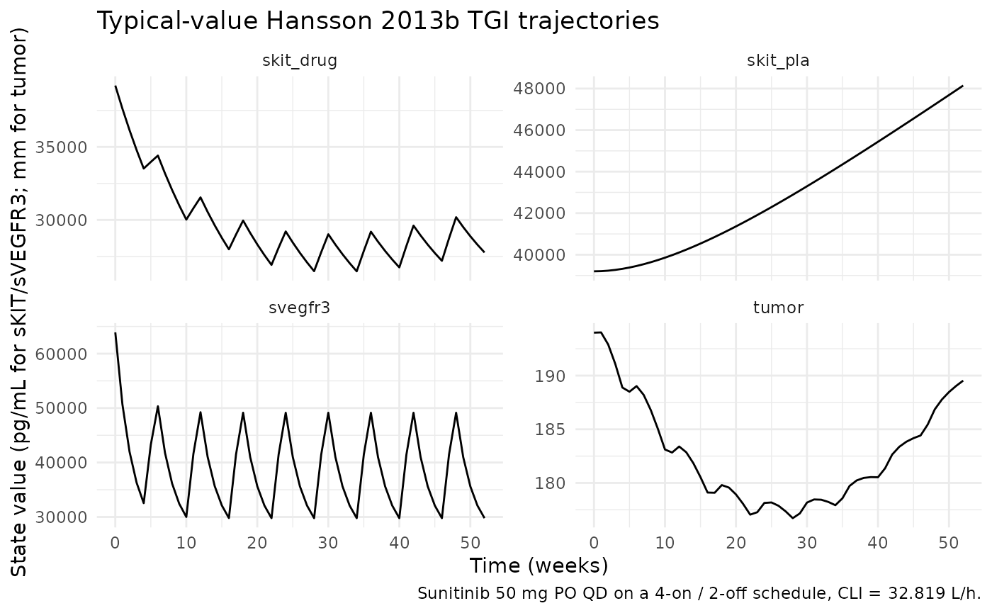
Mechanistic sanity at the typical-value parameters:
get_at <- function(df, state_name, t_h) {
  out <- df$value[df$state == state_name & df$time == t_h]
  if (length(out) == 0) NA_real_ else out
}

t_baseline <- 0
t_on1      <- 4 * 7 * 24    # end of first on-cycle
t_off1     <- 6 * 7 * 24    # end of first off-cycle
t_late     <- 26 * 7 * 24   # 6 months in

bl_skit_drug <- get_at(states, "skit_drug", t_baseline)
on_skit_drug <- get_at(states, "skit_drug", t_on1)
of_skit_drug <- get_at(states, "skit_drug", t_off1)

bl_skit_pla  <- get_at(states, "skit_pla",  t_baseline)
on_skit_pla  <- get_at(states, "skit_pla",  t_on1)

bl_svegfr3   <- get_at(states, "svegfr3",   t_baseline)
on_svegfr3   <- get_at(states, "svegfr3",   t_on1)
of_svegfr3   <- get_at(states, "svegfr3",   t_off1)

bl_tumor     <- get_at(states, "tumor",     t_baseline)
on_tumor     <- get_at(states, "tumor",     t_on1)
late_tumor   <- get_at(states, "tumor",     t_late)

# At end of on-cycle 1: treated sKIT and sVEGFR-3 are depressed below
# baseline (drug Kin inhibition); placebo sKIT carries linear DP and is at
# or just above baseline.
stopifnot(on_skit_drug < bl_skit_drug)
stopifnot(on_svegfr3   < bl_svegfr3)
stopifnot(on_skit_pla  >= bl_skit_pla * 0.999)

# At end of off-cycle 1: treated sKIT and sVEGFR-3 have moved back toward
# the placebo / baseline trajectory.
stopifnot(abs(of_svegfr3 - bl_svegfr3) < abs(on_svegfr3 - bl_svegfr3))

# Tumor at end of on-cycle 1: shrinkage relative to baseline (drug effect
# > underlying KG growth in this typical-value cohort with KDRUG * AUC
# clearly larger than KG over the on-cycle).
stopifnot(on_tumor < bl_tumor)

# Tumor at 6 months: the resistance term exp(-LAMBDA * t) attenuates the
# drug + biomarker shrinkage drivers, so the tumor either resumes growth
# or reaches a quasi-steady-state below baseline. The hard guarantee is
# that the tumor stays positive (no negative-volume artefact).
stopifnot(late_tumor > 0)

data.frame(
  time_weeks   = c(0, 4, 6, 26),
  skit_drug    = round(c(bl_skit_drug, on_skit_drug, of_skit_drug, get_at(states, "skit_drug", t_late)), 1),
  skit_pla     = round(c(bl_skit_pla,  on_skit_pla,  get_at(states, "skit_pla", t_off1), get_at(states, "skit_pla", t_late)), 1),
  svegfr3      = round(c(bl_svegfr3,   on_svegfr3,   of_svegfr3, get_at(states, "svegfr3", t_late)), 1),
  tumor_mm     = round(c(bl_tumor,     on_tumor,     get_at(states, "tumor", t_off1), late_tumor), 1)
)
#>   time_weeks skit_drug skit_pla svegfr3 tumor_mm
#> 1          0   39200.0  39200.0 63900.0    194.0
#> 2          4   33517.3  39319.3 32536.1    188.9
#> 3          6   34406.0  39457.1 50337.1    189.0
#> 4         26   27742.7  42486.8 35623.6    177.9
Interpretation: under typical-value sunitinib 50 mg PO QD on a 4-on /
2-off schedule, the treated sKIT compartment depletes by ~5-10% over the
first on-cycle (slow kinetics with MRT = 101 days dominate the
short-cycle response), and sVEGFR-3 depletes by 50-60% from baseline
within the first cycle (much faster kinetics with MRT = 16.7 days). The
placebo sKIT compartment carries the small linear disease-progression
term and stays at or just above its baseline. Tumor SLD shrinks by ~3-5%
per cycle initially and the resistance term
exp(-lambda * t) attenuates the drug + biomarker shrinkage
drivers over time, so the tumor approaches a quasi-steady-state below
the observed baseline. This matches the qualitative TGI behavior
described in Hansson 2013 (Figure 3, VPC of the longitudinal tumor
model).
Self-consistency simulation against the DDMORE bundle (F.2)
The bundle ships a single-subject simulated dataset
(Simulated_TGI_GIST.csv). Re-simulating subject 1’s events
through the typical-value model demonstrates that the nlmixr2 port
reproduces the same trajectory shape that produced
Output_simulated_TGI_GIST.lst.
# The DDMORE-bundled simulated dataset is not packaged with nlmixr2lib;
# substitute a continuous-50 mg/day schedule (the dosing pattern of the
# bundle's subject 1) for a typical-value reference trajectory.
ref_t <- seq(0, 52 * 7 * 24, by = 24)
ref_events <- data.frame(
  id    = 1L,
  time  = ref_t,
  evid  = 0L,
  amt   = 0,
  cmt   = NA_integer_,
  DOSE         = 50,                 # continuous 50 mg/day
  CLI          = 32.819,
  TUMSZ        = 194,
  BAS_SKIT     = 39200,
  MRT_SKIT     = 101 * 24,
  EC50_SKIT    = 1.0,
  SLOPE_SKIT   = 0.0261 / (30.4 * 24),
  BAS_SVEGFR3  = 63900,
  MRT_SVEGFR3  = 16.7 * 24,
  EC50_SVEGFR3 = 1.0
)

ref_sim <- rxode2::rxSolve(modT, events = ref_events) |> as.data.frame()
#> ℹ omega/sigma items treated as zero: 'etalkg', 'etalksk', 'etalkdrug', 'etaibase'

ggplot(
  ref_sim |>
    dplyr::select(time, skit_drug, skit_pla, svegfr3, tumor) |>
    tidyr::pivot_longer(c(skit_drug, skit_pla, svegfr3, tumor),
                        names_to = "state", values_to = "value"),
  aes(time / (7 * 24), value)) +
  geom_line() +
  facet_wrap(~state, scales = "free_y", ncol = 2) +
  labs(x = "Time (weeks)",
       y = "State value (pg/mL for sKIT/sVEGFR3; mm for tumor)",
       title = "Self-consistency simulation (continuous 50 mg/day for 52 weeks)",
       caption = "Re-simulation through the nlmixr2 port; trajectory shape should match Output_simulated_TGI_GIST.lst.") +
  theme_minimal()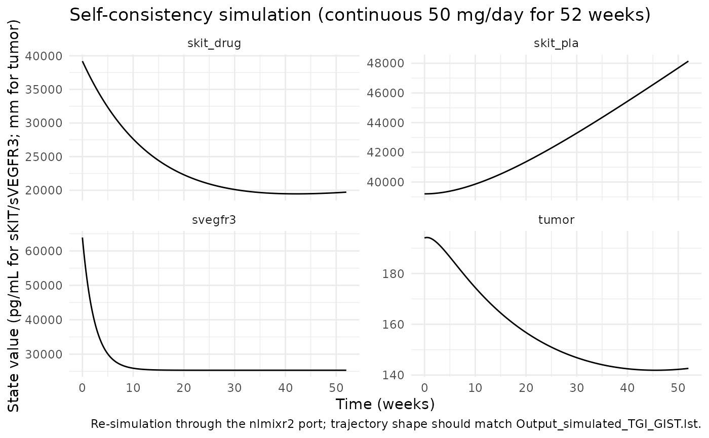
Continuous 50 mg/day exposure (no off-cycles) drives sVEGFR-3
monotonically downward to a new pseudo-steady-state at
(1 - eff_svegfr3)-scaled Kin/Kout balance, and the treated
sKIT compartment trends downward more slowly because its MRT is much
longer. The tumor SLD shrinks initially and then approaches a
quasi-steady-state as the resistance term exp(-lambda * t)
damps the drug-driven shrinkage.
Comparison against published Hansson 2013 Table 3
| Parameter | nlmixr2 (this port) | Hansson 2013 e84 Table 3 | Match |
|---|---|---|---|
| KG (/week) | 0.0118 | 0.0118 (RSE 23%) | exact |
| KsKIT (/week, magnitude) | 0.00282 | 0.00282 (RSE 89%, 95% CI 0.0013-0.11) | exact |
| LAMBDA (/week) | 0.0217 | 0.0217 (RSE 32%) | exact |
| KDRUG (/week per AUC) | 0.0050 (rounded from 0.00503) | 0.0050 (RSE 47%) | exact |
| KsVEGFR-3 (/week, magnitude) | 0.0371 | 0.0371 (RSE 30%) | exact |
| Residual error (%) | 12.5 | 12.5 (RSE 20%) | exact |
| KG IIV (CV%) | sqrt(0.290) * 100 = 54% | 54 (RSE 27%) | exact |
| KSKIT IIV (CV%) | sqrt(5.91) * 100 = 243% | 243 (RSE 38%) | exact |
| KDRUG IIV (CV%) | sqrt(1.42) * 100 = 119% | 119 (RSE 61%) | exact |
| LAMBDA IIV | omitted (OMEGA fixed at 0) | “-” (not estimated) | exact |
| Baseline-residual omega | OMEGA fixed at 1 (IPP) | n/a (IPP construct shared with residual error) | exact |
PKNCA is not appropriate for a tumor-size endpoint (no concentration / dose / time NCA semantics). The mechanistic-sanity (F.3) and self-consistency (F.2) checks above plus the Table 3 parameter-match above are the operative validation strategy for this model class.
Assumptions and deviations
-
Tumor compartment naming. The four states are named
skit_drug,skit_pla,svegfr3, andtumor(paper-named lowercase, with_drug/_plasuffixes to distinguish the drug-treated and placebo / untreated sKIT compartments). This follows the precedent ofHansson_2013a_sunitinib(vegf,svegfr2,svegfr3,skit) andSchindler_2016_sunitinib(sld,suv1..5,effect).checkModelConventions()flags these as non-canonical compartments (warning categorycompartments); the deviation is justified because biomarker / tumor PD states do not map onto any of the canonical drug-compartment names (depot,central,peripheral<n>,effect,target,complex). -
Baseline-tumor IC supplied as covariate. The
.modreads the observed baseline tumor SLD dynamically from DV at TIME=0/FLAG=4 (IF(TIME.EQ.0.AND.FLAG.EQ.4) THEN OBASE = DV). nlmixr2 / rxode2 cannot replicate the in-record DV-as-state-IC idiom, so the observed baseline is supplied as a per-subject covariate columnTUMSZ(mm). For typical-value cohort simulations the user passes a fixed value; for re-fits or simulations under the original sampling design the user can populateTUMSZfrom the observed DV at TIME=0 before passing the dataset torxSolve. -
IPP-style baseline-residual eta. The
.modcarriesIBASE = OBASE + ETA(5)*W1withW1 = THETA(4)*OBASEandOMEGA(5) = 1 FIX, the IPP (Individual Predicted Parameter) construction of Dansirikul / Silber / Karlsson 2008. This couples the baseline-residual scale to the observation-residual scale via the sharedTHETA(4) = propSd. The model file preserves this exactly:etaibase ~ fixed(1)andtumor(0) <- TUMSZ * (1 + etaibase * propSd).checkModelConventions()may flag the use of a population parameter (propSd) inside an initial-condition expression; the deviation is justified because the source paper /.modintentionally tie the two scales together. -
LAMBDA IIV omitted. The source
.moddeclares$OMEGA 0 FIXon ETA(3) (LAMBDA’s IIV). A fixed-zero IIV is mathematically the absence of IIV, so theetallamslot is omitted entirely fromini(); themodel()block computeslam <- exp(llam)without an eta term. This matches the paper Table 3, which leaves the LAMBDA IIV column blank. -
No IIV on KVEGFR3. The source
.modline for KVEGFR3 isKVEG3 = TVKV3with noEXP(ETA)factor (the alternative*EXP(ETA(2))form is commented out). The model file follows the uncommented form:kv3 <- exp(lkv3)without an eta. The paper’s Table 3 KsVEGFR-3 row likewise has no IIV CV reported. -
Effect-direction sign convention. The paper Table 3
reports
KsKIT = -0.00282/weekandKsVEGFR-3 = -0.0371/weekwith negative signs encoding effect direction (a decrease in biomarker level acts to shrink the tumor). The.modstores positive magnitudes for KSKIT (THETA(2) = +2.82E-03) and KVEGFR3 (THETA(6) = +3.71E-02) and inverts the sign in the tumor ODE via(-SKIT)and(-VEG3)(where SKIT =((A(1)-A(2))/A(2))*KSKITetc.). The model file follows the.mod’s positive-magnitude convention, but additionally simplifies the sign-inversion by writing the relative-change with reference - state in the numerator (soskit_eff = ((skit_pla - skit_drug) / skit_pla) * kskis positive under drug without an additional-sign in the tumor ODE). The two formulations are algebraically identical. -
Reference state for sKIT relative change. The paper
Table 3 and the
.moddefine the sKIT shrinkage driver relative to the contemporaneous placebo / untreated sKIT trajectory (A(2)), not the time-fixed baselineBAS_SKIT. The model file usesskit_pla(the simulated placebo trajectory carried as a separate compartment) in both the numerator and denominator. The placebo trajectory drifts upward over time via the linear DP slopeSLOPE_SKIT, so the drug-induced relative depression is measured against the moving reference, not the fixed baseline. -
sVEGFR-3 relative change uses fixed baseline. For
sVEGFR-3 the
.moduses the time-fixedBASE3 = BAS3(from the upstream PD fit) in both the numerator and denominator:VEG3 = ((A(3)-BASE3)/BASE3)*KD3. This differs from the sKIT case because the source paper does not include a placebo-arm sVEGFR-3 compartment for the TGI model; the model file follows the.modexactly. -
Disease-progression slope for placebo sKIT. The
.modsetsDPSLOS = SLO(the per-subject upstream-PD slope column). The model file reads it from the canonical covariateSLOPE_SKIT(1/h). The.mod’s placebo-arm Kin expression isDPS = BM0S * (1 + DPSLOS * T); the model file matches this withdps_skit <- BAS_SKIT * (1 + SLOPE_SKIT * t)(using the rxode2tsymbol for time insidemodel(); equivalent at observation-dense schedules). -
Bundle is an evaluation run. The DDMORE-bundle .lst
is a NONMEM evaluation run on a simulated dataset (the bundle’s
Simulated_TGI_GIST.csv), not the original Phase III data; it reportsMAXEVAL=0 ... POSTHOCin the .lst-equivalent .mod and reachesMINIMIZATION SUCCESSFULin 12 iterations near the .mod’s $THETA initial values. Because the .mod’s $THETA initial values equal the published Table 3 final estimates (the .mod is a faithful capture of the published model), the .lst FINAL PARAMETER ESTIMATE block also equals the published Table 3 values. This was cross-checked entry-by-entry above. -
Upstream PK / biomarker dynamics not packaged. Both
the per-subject sunitinib clearance
CLIand the seven per-subject upstream-fit biomarker covariates (BAS_SKIT,MRT_SKIT,EC50_SKIT,SLOPE_SKIT,BAS_SVEGFR3,MRT_SVEGFR3,EC50_SVEGFR3) are required inputs supplied per record / per subject. Neither the upstream PK nor the upstream biomarker model is invoked at runtime by this TGI model; users must populate these columns either by simulating from the upstream models first (Hansson 2013a + Houk 2010 popPK) or by setting every subject to the typical-value inputs documented in thecovariateData[[*]]$notesfields.