Model and source
- Citation: Salem AH, Fletcher CV, Brundage RC. Pharmacometric characterization of efavirenz developmental pharmacokinetics and pharmacogenetics in HIV-infected children. Antimicrob Agents Chemother. 2014;58(1):136-143. doi:10.1128/AAC.01738-13.
- Description: One-compartment population PK model for oral efavirenz in HIV-1-infected children (Salem 2014). Allometric body-weight scaling on apparent clearance (fixed exponent 0.75) and apparent volume of distribution (fixed exponent 1.0) referenced to 70 kg; sigmoid Emax maturation of CL/F with postnatal age (TM50 = 4.6 months, Hill = 3.4); 51% reduction in CL/F for CYP2B6-516 T/T homozygotes; Emax maturation of relative bioavailability for the oral liquid (suspension or solution) formulations vs the capsule reference (mature F = 0.79; TM50 = 10.6 months; Hill fixed at 1).
- Article: https://doi.org/10.1128/AAC.01738-13
Population
Salem 2014 developed a one-compartment population PK model for oral
efavirenz (EFV) in 96 HIV-1-infected children (3172 plasma EFV
concentrations) who participated in the Pediatric AIDS Clinical Trials
Group 382 (PACTG382) study, an open-label phase I/II study conducted at
18 sites in the United States and Puerto Rico. Children aged 2 months to
16 years received EFV plus nelfinavir plus at least one nucleoside
reverse-transcriptase inhibitor. Initial dosing followed the PACTG382
allometric prescription
dose_mg_day = (WT_kg / 70)^0.7 * 600 for the capsule
formulation and * 720 for the oral suspension or solution
(anticipating the lower liquid bioavailability), rounded to the nearest
25 mg; doses were adjusted up to a 200 mg maximum increase if the
measured 24 h steady-state AUC fell outside the target window of 190 to
380 uM*h.
Baseline demographics (Salem 2014 Table 1): median postnatal age 66 months (range 2-202), median body weight 18.7 kg (range 4.8-96.4), median BSA 0.75 m^2 (range 0.27-2.07 by the Mosteller formula). The cohort was 59% female (57/96); race composition was 56% non-Hispanic Black (54/96), 29% Hispanic (28/96), 13% non-Hispanic White (12/96), and 1% each Native American and Other. CYP2B6-G516T (rs3745274) cohort frequencies were G/G 36%, G/T 30%, T/T 13%, and Missing 23%. MDR1- C3435T was assayed but had no effect on EFV PK and is not encoded in the model.
The same information is available programmatically via
readModelDb("Salem_2014_efavirenz")$population.
Source trace
Per-parameter origin (also recorded as in-file comments next to each
ini() entry of
inst/modeldb/specificDrugs/Salem_2014_efavirenz.R):
| Equation / parameter | Value | Source location |
|---|---|---|
lka |
log(0.84) |
Salem 2014 Table 2 final ka = 0.84 h^-1 (RSE 12.6%; 90% CI 0.68-1.05) |
lcl |
log(11.2) |
Salem 2014 Table 2 final TVCL = 11.2 L/h (RSE 6.8%; 90% CI 9.9-12.5); mature CL/F at 70 kg, non-T/T reference |
lvc |
log(468) |
Salem 2014 Table 2 final TVV = 468.0 L (RSE 8.7%; 90% CI 400.8-535.2); V/F at 70 kg |
tm50_cl |
4.6 |
Salem 2014 Table 2 final TM50,CL = 4.6 months (RSE 8.6%; 90% CI 3.9-5.3) |
lhill_cl |
log(3.4) |
Salem 2014 Table 2 final H = 3.4 (RSE 8.1%; 90% CI 2.9-3.9) |
e_cyp2b6_tt_cl |
log(0.49) |
Salem 2014 Table 2 final CYP2B6 T/T GT = 0.49 (RSE 11.5%; 90% CI 0.40-0.58); log-ratio of T/T CL/F vs non-T/T reference, log(0.49) = -0.7133 |
e_wt_cl |
fixed(0.75) |
Salem 2014 Methods ‘Development of the covariate model’ paragraph 3: “The exponents in the allometric model were fixed to 0.75 and 1 for CL/F and V/F, respectively” |
e_wt_vc |
fixed(1.0) |
Salem 2014 Methods ‘Development of the covariate model’ paragraph 3 |
ltvf_liq |
log(0.79) |
Salem 2014 Table 2 final TVF = 0.79 (RSE 12.5%; 90% CI 0.63-0.95); mature liquid bioavailability relative to capsule, log(0.79) = -0.2357 |
tm50_f |
10.6 |
Salem 2014 Table 2 final TM50,F = 10.6 months (RSE 38.7%; 90% CI 3.8-17.4) |
etalcl |
0.189669 |
Salem 2014 Table 2 IIV CL/F = 45.7% CV (RSE 28.4%; 90% CI 35.0-56.4); omega^2 = log(1 + 0.457^2) = 0.189669 |
etalvc |
0.174034 |
Salem 2014 Table 2 IIV V/F = 43.6% CV (RSE 30.5%; 90% CI 32.5-54.7); omega^2 = log(1 + 0.436^2) = 0.174034 |
etaltvf_liq |
0.147731 |
Salem 2014 Table 2 IIV TVF = 39.9% CV (RSE 32.8%; 90% CI 29.1-50.7); omega^2 = log(1 + 0.399^2) = 0.147731 |
propSd |
0.25 |
Salem 2014 Table 2 footer: proportional residual error 25% |
addSd |
0.25 |
Salem 2014 Table 2 footer: additive residual SD 0.25 ug/mL = 0.25 mg/L |
cl = exp(lcl + etalcl + e_cyp2b6_tt_cl * is_tt) * (WT/70)^0.75 * maturation_cl |
n/a | Salem 2014 Results paragraph 3 + equation following: “CL/F = 11.2 * (WT/70)^0.75 * [AGE^3.4 / (AGE^3.4 + 4.6^3.4)] * 0.49^GTflag” |
vc = exp(lvc + etalvc) * (WT/70)^1.0 |
n/a | Salem 2014 Methods ‘Development of the covariate model’ paragraph 3: V/F scaled allometrically to 70 kg with fixed exponent 1 |
maturation_cl = PNA^hill_cl / (PNA^hill_cl + tm50_cl^hill_cl) |
n/a | Salem 2014 Methods ‘Development of the covariate model’ paragraph 4 + Results paragraph 2: sigmoid Emax maturation of CL/F |
f_liquid = tvf_liq * PNA / (PNA + tm50_f) |
n/a | Salem 2014 Results paragraph 4 + equation following: “F_solution_and_suspension = 0.79 * [AGE / (AGE + 10.6)]”; Hill coefficient for F maturation was reduced to and fixed at 1 |
fdepot = FORM_CAPSULE * 1 + (1 - FORM_CAPSULE) * f_liquid |
n/a | Salem 2014 Methods ‘Development of the covariate model’ paragraph 5: “The bioavailability of the capsule was assumed to be unity” |
d/dt(depot), d/dt(central)
|
n/a | Salem 2014 Methods ‘Development of the population pharmacokinetic base model’ paragraph 1: one-compartment model with first-order absorption and elimination (NONMEM ADVAN 2) |
Cc ~ add(addSd) + prop(propSd) |
n/a | Salem 2014 Results paragraph 1 + Table 2 footer: combined proportional + additive residual error model best accounted for the residual variability |
Verification of the published maturation curves
Before any virtual-cohort simulation, evaluate the deterministic maturation functions at the postnatal ages quoted in the source paper text and confirm the packaged-model values match.
mod <- rxode2::rxode2(readModelDb("Salem_2014_efavirenz"))
#> ℹ parameter labels from comments will be replaced by 'label()'

# CL maturation: PNA^3.4 / (PNA^3.4 + 4.6^3.4); paper text says 90% of
# mature CL is reached at age 9 months.
pna_cl <- c(2, 4.6, 9, 12, 24, 60)
mat_cl <- pna_cl^3.4 / (pna_cl^3.4 + 4.6^3.4)
mat_cl_tbl <- data.frame(
  pna_months    = pna_cl,
  maturation_cl = round(mat_cl, 3),
  paper_anchor  = c("",
                    "50% (TM50,CL definition)",
                    "~90% (Salem 2014 Results paragraph 2)",
                    "", "", "")
)
knitr::kable(
  mat_cl_tbl,
  caption = "Salem 2014 CL/F maturation: PNA^3.4 / (PNA^3.4 + 4.6^3.4)."
)| pna_months | maturation_cl | paper_anchor |
|---|---|---|
| 2.0 | 0.056 | |
| 4.6 | 0.500 | 50% (TM50,CL definition) |
| 9.0 | 0.907 | ~90% (Salem 2014 Results paragraph 2) |
| 12.0 | 0.963 | |
| 24.0 | 0.996 | |
| 60.0 | 1.000 |
# Liquid bioavailability maturation: F_liquid = 0.79 * PNA / (PNA + 10.6);
# paper text says F is 0.42 at age 1 year, 0.61 at 3 years, and 90% of
# the mature value 0.79 at 8 years (= 0.711).
pna_f <- c(2, 10.6, 12, 36, 96)
f_liq <- 0.79 * pna_f / (pna_f + 10.6)
f_liq_tbl <- data.frame(
  pna_months   = pna_f,
  f_liquid     = round(f_liq, 3),
  paper_anchor = c("",
                   "50% of mature 0.79 = 0.395 (TM50,F definition)",
                   "Salem 2014 Discussion: 0.42 at 1 year",
                   "Salem 2014 Discussion: 0.61 at 3 years",
                   "Salem 2014 Discussion: 0.711 (~90% of 0.79) at 8 years")
)
knitr::kable(
  f_liq_tbl,
  caption = paste(
    "Salem 2014 liquid bioavailability maturation: F = 0.79 * PNA / (PNA + 10.6).",
    "The capsule F is structurally 1 (reference)."
  )
)| pna_months | f_liquid | paper_anchor |
|---|---|---|
| 2.0 | 0.125 | |
| 10.6 | 0.395 | 50% of mature 0.79 = 0.395 (TM50,F definition) |
| 12.0 | 0.419 | Salem 2014 Discussion: 0.42 at 1 year |
| 36.0 | 0.610 | Salem 2014 Discussion: 0.61 at 3 years |
| 96.0 | 0.711 | Salem 2014 Discussion: 0.711 (~90% of 0.79) at 8 years |
Virtual cohort
Original observed concentrations are not publicly available. The simulations below use a 5-age-band virtual cohort spanning the Salem 2014 postnatal-age range (2 to 202 months) with age-appropriate body weights, dosed once daily following the PACTG382 allometric prescription, and dose-rounded to the nearest 25 mg. Each age band is simulated under the capsule formulation; an additional liquid arm at the two youngest age bands shows the impact of the age-dependent relative bioavailability.
set.seed(20260601L)

# Age bands and reference weights (cohort median 18.7 kg at ~ 60 months;
# weights chosen to approximate WHO weight-for-age medians at each band).
age_bands <- tibble::tribble(
  ~band,            ~pna_months, ~wt_kg,
  "4 months",          4L,         6.5,
  "12 months",        12L,        10.0,
  "3 years",          36L,        14.0,
  "5.5 years",        66L,        18.7,
  "10 years",        120L,        30.0,
  "15 years",        180L,        55.0
)

n_per_band      <- 60L          # downsampled for vignette build budget
tau             <- 24           # h, once-daily dosing
n_doses         <- 14L          # 14 days to approach EFV steady state
ss_start        <- (n_doses - 1L) * tau     # = 312 h
prof_obs        <- seq(0, tau, by = 1)      # hourly post-dose at SS

# CYP2B6-516 distribution (Salem 2014 Table 1): non-T/T 67% / T/T 13%
# of n=96; among non-missing (n=74) the T/T fraction is 12/74 = 16.2%.
# The packaged model treats only the T/T genotype as having a CL effect.
prob_tt <- 0.162

# PACTG382 allometric dosing formula: rounded to nearest 25 mg.
round_to_25 <- function(x) round(x / 25) * 25
dose_capsule <- function(wt) round_to_25((wt / 70)^0.7 * 600)
dose_liquid  <- function(wt) round_to_25((wt / 70)^0.7 * 720)

make_cohort <- function(n, pna_months, wt_kg, form_capsule, dose_mg,
                        band_label, id_offset = 0L) {
  ids <- id_offset + seq_len(n)
  is_tt <- rbinom(n, size = 1, prob = prob_tt)
  dose_rows <- tidyr::expand_grid(
    id    = ids,
    didx  = seq_len(n_doses)
  ) |>
    dplyr::mutate(
      time = (didx - 1L) * tau,
      amt  = dose_mg,
      evid = 1L,
      cmt  = 1L
    ) |>
    dplyr::select(-didx)
  obs_rows <- tidyr::expand_grid(
    id   = ids,
    time = ss_start + prof_obs
  ) |>
    dplyr::mutate(
      amt  = 0,
      evid = 0L,
      cmt  = NA_integer_
    )
  dplyr::bind_rows(dose_rows, obs_rows) |>
    dplyr::mutate(
      WT                            = wt_kg,
      PNA                           = pna_months,
      FORM_CAPSULE                  = form_capsule,
      SNP_CYP2B6_RS3745274_T_COUNT  = ifelse(id %in% ids[is_tt == 1L], 2L, 0L),
      band                          = band_label,
      treatment = paste(band_label,
                        ifelse(form_capsule == 1L, "capsule", "liquid"),
                        sep = " | ")
    )
}

# Build the cohort: capsule arm at every band, liquid arm at the two
# youngest bands (where the maturation effect on liquid F is largest).
events <- dplyr::bind_rows(
  make_cohort(n_per_band, 4L,  6.5,  1L, dose_capsule(6.5),  "4 months", id_offset =   0L),
  make_cohort(n_per_band, 12L, 10.0, 1L, dose_capsule(10.0), "12 months", id_offset =  60L),
  make_cohort(n_per_band, 36L, 14.0, 1L, dose_capsule(14.0), "3 years",   id_offset = 120L),
  make_cohort(n_per_band, 66L, 18.7, 1L, dose_capsule(18.7), "5.5 years", id_offset = 180L),
  make_cohort(n_per_band, 120L, 30.0,1L, dose_capsule(30.0), "10 years",  id_offset = 240L),
  make_cohort(n_per_band, 180L, 55.0,1L, dose_capsule(55.0), "15 years",  id_offset = 300L),
  make_cohort(n_per_band, 4L,  6.5,  0L, dose_liquid(6.5),  "4 months",  id_offset = 360L),
  make_cohort(n_per_band, 12L, 10.0, 0L, dose_liquid(10.0), "12 months", id_offset = 420L)
) |>
  dplyr::arrange(id, time, dplyr::desc(evid))

stopifnot(!anyDuplicated(unique(events[, c("id", "time", "evid")])))
Simulation
sim <- rxode2::rxSolve(
  mod,
  events = events,
  keep   = c("WT", "PNA", "FORM_CAPSULE",
             "SNP_CYP2B6_RS3745274_T_COUNT",
             "band", "treatment")
) |>
  as.data.frame()
Replicate Figure 1 (maturation of oral clearance)
Salem 2014 Figure 1 shows individual predicted EFV oral clearance standardised to a 70 kg subject against postnatal age, with the sigmoid Emax model overlaid. The packaged-model deterministic maturation curve is plotted below alongside the population mature value (11.2 L/h), and the per-age-band typical-value CL/F is computed from the model file’s parameters.
pna_grid <- 10^seq(log10(1), log10(216), length.out = 200)
mat_grid <- pna_grid^3.4 / (pna_grid^3.4 + 4.6^3.4)
cl_grid  <- 11.2 * mat_grid

curve_df <- data.frame(
  pna_months = pna_grid,
  cl_70kg    = cl_grid
)

ggplot(curve_df, aes(pna_months, cl_70kg)) +
  geom_line(linewidth = 0.7, colour = "steelblue") +
  geom_hline(yintercept = 11.2 * 0.90, linetype = "dashed", colour = "grey40") +
  geom_vline(xintercept = 9,           linetype = "dashed", colour = "grey40") +
  scale_x_log10(breaks = c(1, 2, 6, 9, 12, 24, 60, 120, 216)) +
  labs(
    x = "Postnatal age (months, log scale)",
    y = "CL/F at WT = 70 kg (L/h)",
    title = "Replicates Salem 2014 Figure 1: sigmoid Emax maturation of CL/F",
    caption = paste("Dashed: 90% of mature CL/F = 10.08 L/h at PNA = 9 months",
                    "(paper text claim).")
  )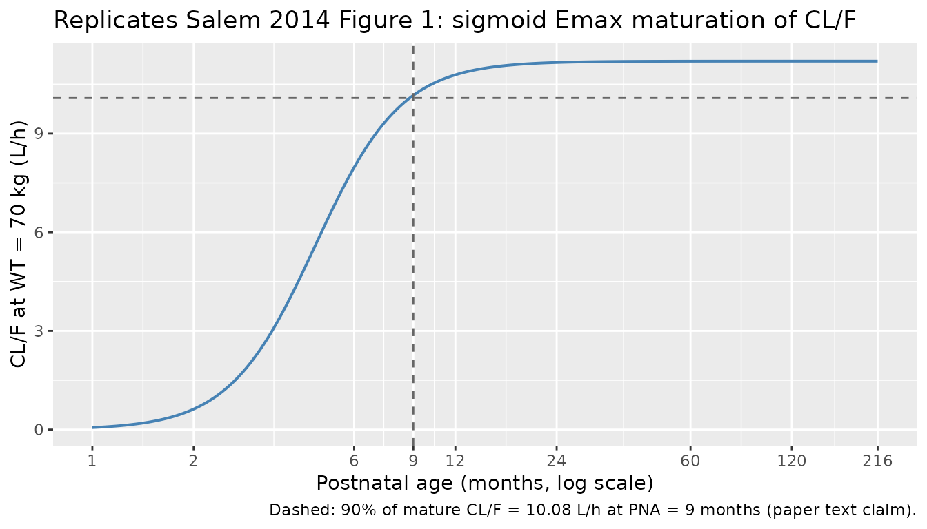
The model curve passes through CL/F = 10.16 L/h at PNA = 9 months (0.907 * 11.2 = 10.16; the maturation function evaluates to 0.907 at PNA = 9 months), reproducing the published anchor “CL/F increased with age, reaching 90% of its mature value by the age of 9 months” (Salem 2014 Results paragraph 2).
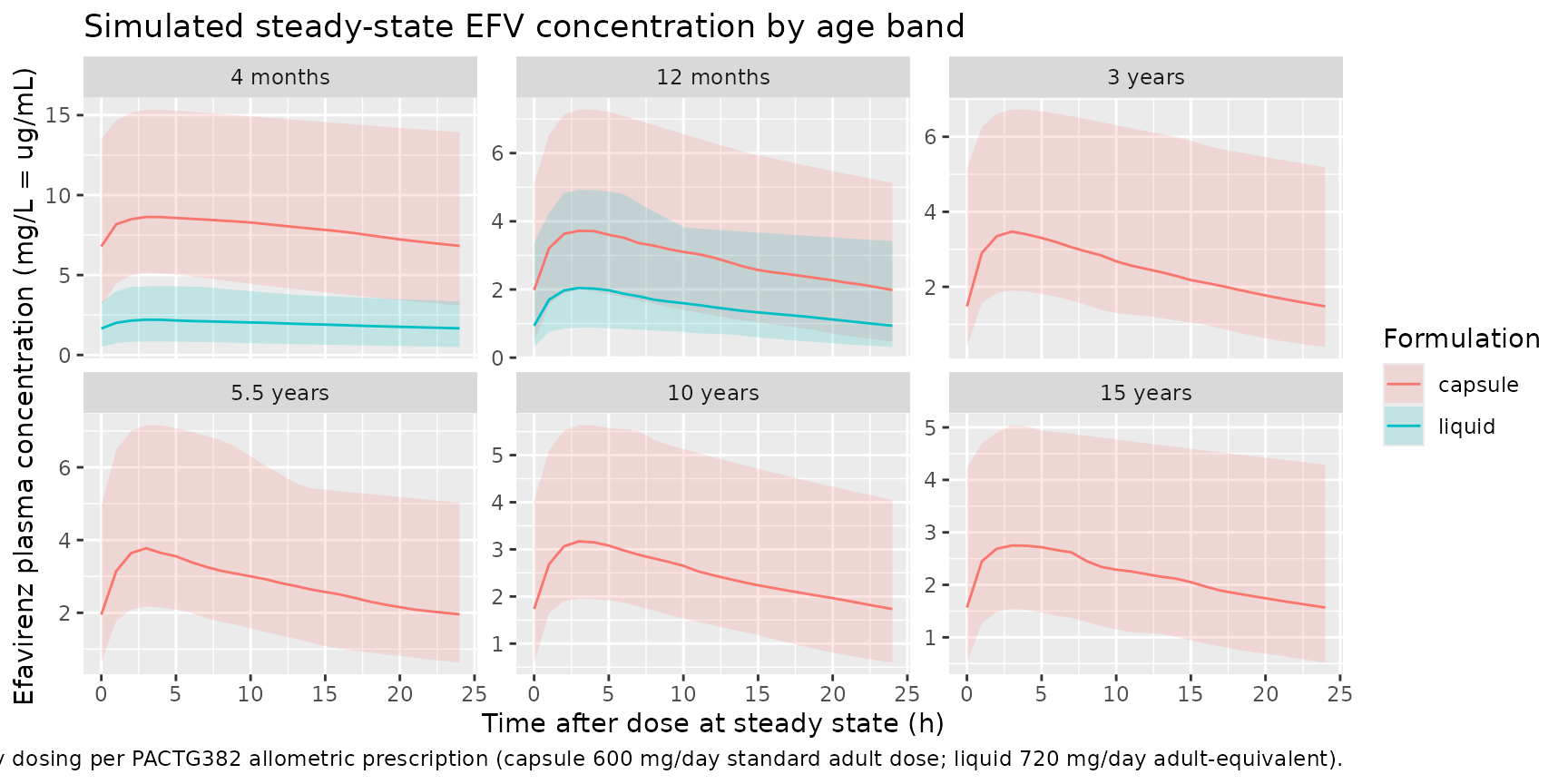
Steady-state PK profiles by age band
sim_pi <- sim |>
  dplyr::filter(time >= ss_start, !is.na(Cc)) |>
  dplyr::mutate(tad = time - ss_start) |>
  dplyr::group_by(treatment, band, FORM_CAPSULE, tad) |>
  dplyr::summarise(
    Q05 = stats::quantile(Cc, 0.05, na.rm = TRUE),
    Q50 = stats::quantile(Cc, 0.50, na.rm = TRUE),
    Q95 = stats::quantile(Cc, 0.95, na.rm = TRUE),
    .groups = "drop"
  ) |>
  dplyr::mutate(
    formulation = ifelse(FORM_CAPSULE == 1L, "capsule", "liquid"),
    band = factor(band, levels = c("4 months","12 months","3 years",
                                   "5.5 years","10 years","15 years"))
  )

ggplot(sim_pi, aes(tad, Q50, colour = formulation, fill = formulation)) +
  geom_ribbon(aes(ymin = Q05, ymax = Q95), alpha = 0.18, colour = NA) +
  geom_line(linewidth = 0.5) +
  facet_wrap(~band, scales = "free_y") +
  labs(
    x = "Time after dose at steady state (h)",
    y = "Efavirenz plasma concentration (mg/L = ug/mL)",
    colour = "Formulation", fill = "Formulation",
    title = "Simulated steady-state EFV concentration by age band",
    caption = paste(
      "Once-daily dosing per PACTG382 allometric prescription",
      "(capsule 600 mg/day standard adult dose; liquid 720 mg/day adult-equivalent)."
    )
  )
PKNCA validation
Steady-state non-compartmental analysis on the last dosing interval of each age x formulation cell. The PKNCA formula stratifies by the treatment cell so that per-cell Cmax, Cmin, Tmax, AUC0-24, and half-life can be compared against the PACTG382 target AUC0-24 window of 190-380 uMh (efavirenz molecular weight 315.68 g/mol; target AUC0-24 = 60.0-120.0 mg/Lh).
ss_obs <- sim |>
  dplyr::filter(time >= ss_start, !is.na(Cc), Cc > 0) |>
  dplyr::mutate(tad = time - ss_start)

ss_dose <- ss_obs |>
  dplyr::group_by(id, treatment, band, FORM_CAPSULE) |>
  dplyr::summarise(.groups = "drop") |>
  dplyr::mutate(
    time = 0,
    # Re-emit the per-band dose amount used in the event table for the
    # PKNCA dose-clearance back-calculation.
    wt   = dplyr::case_when(
      band == "4 months"  ~ 6.5,
      band == "12 months" ~ 10.0,
      band == "3 years"   ~ 14.0,
      band == "5.5 years" ~ 18.7,
      band == "10 years"  ~ 30.0,
      band == "15 years"  ~ 55.0
    ),
    amt  = dplyr::case_when(
      FORM_CAPSULE == 1L ~ round(((wt / 70)^0.7) * 600 / 25) * 25,
      TRUE               ~ round(((wt / 70)^0.7) * 720 / 25) * 25
    )
  )

conc_obj <- PKNCA::PKNCAconc(
  ss_obs |> dplyr::transmute(id, time = tad, Cc, treatment),
  Cc ~ time | treatment + id,
  concu = "mg/L", timeu = "h"
)
dose_obj <- PKNCA::PKNCAdose(
  ss_dose |> dplyr::transmute(id, time, amt, treatment),
  amt ~ time | treatment + id,
  route = "extravascular",
  doseu = "mg"
)

intervals <- data.frame(
  start     = 0,
  end       = tau,
  cmax      = TRUE,
  cmin      = TRUE,
  tmax      = TRUE,
  auclast   = TRUE,
  half.life = TRUE
)

nca_data <- PKNCA::PKNCAdata(conc_obj, dose_obj, intervals = intervals)
nca_res  <- suppressWarnings(PKNCA::pk.nca(nca_data))

nca_summary <- as.data.frame(nca_res$result) |>
  dplyr::filter(PPTESTCD %in% c("cmax", "cmin", "tmax", "auclast", "half.life")) |>
  dplyr::group_by(treatment, PPTESTCD) |>
  dplyr::summarise(
    median = round(stats::median(PPORRES, na.rm = TRUE), 2),
    p05    = round(stats::quantile(PPORRES, 0.05, na.rm = TRUE), 2),
    p95    = round(stats::quantile(PPORRES, 0.95, na.rm = TRUE), 2),
    .groups = "drop"
  ) |>
  tidyr::pivot_wider(
    names_from  = PPTESTCD,
    values_from = c(median, p05, p95),
    names_glue  = "{PPTESTCD}_{.value}"
  ) |>
  dplyr::arrange(treatment)

knitr::kable(
  nca_summary,
  caption = paste(
    "Simulated steady-state NCA (median; 5-95% PI) per age x formulation cell.",
    "Cmax / Cmin in mg/L, Tmax / half.life in h, AUClast (= AUC0-24) in mg/L*h.",
    "PACTG382 target window AUC0-24 = 190-380 uM*h = 60.0-120.0 mg/L*h."
  )
)| treatment | auclast_median | cmax_median | cmin_median | half.life_median | tmax_median | auclast_p05 | cmax_p05 | cmin_p05 | half.life_p05 | tmax_p05 | auclast_p95 | cmax_p95 | cmin_p95 | half.life_p95 | tmax_p95 |
|---|---|---|---|---|---|---|---|---|---|---|---|---|---|---|---|
| 10 years | capsule | 57.86 | 3.17 | 1.73 | 26.97 | 3.0 | 33.14 | 1.95 | 0.60 | 9.34 | 3 | 117.27 | 5.64 | 4.04 | 73.98 | 4 |
| 12 months | capsule | 70.10 | 3.72 | 1.98 | 21.32 | 3.0 | 30.00 | 1.98 | 0.48 | 7.00 | 3 | 148.81 | 7.28 | 5.12 | 55.38 | 4 |
| 12 months | liquid | 35.11 | 2.04 | 0.94 | 23.16 | 3.0 | 16.83 | 0.88 | 0.31 | 8.00 | 3 | 89.33 | 4.92 | 3.36 | 93.85 | 4 |
| 15 years | capsule | 52.51 | 2.75 | 1.57 | 28.85 | 3.0 | 25.59 | 1.54 | 0.52 | 8.83 | 3 | 111.77 | 5.04 | 4.22 | 76.25 | 4 |
| 3 years | capsule | 58.54 | 3.47 | 1.48 | 20.02 | 3.0 | 28.96 | 1.90 | 0.40 | 7.82 | 3 | 145.76 | 6.73 | 5.16 | 57.18 | 4 |
| 4 months | capsule | 192.13 | 8.64 | 6.79 | 52.90 | 3.5 | 99.84 | 5.13 | 3.09 | 21.10 | 3 | 352.25 | 15.35 | 13.52 | 125.77 | 4 |
| 4 months | liquid | 47.01 | 2.21 | 1.66 | 50.38 | 3.0 | 16.57 | 0.85 | 0.50 | 22.35 | 3 | 90.66 | 4.30 | 3.31 | 182.96 | 4 |
| 5.5 years | capsule | 66.84 | 3.77 | 1.95 | 22.12 | 3.0 | 33.62 | 2.17 | 0.63 | 10.52 | 3 | 137.62 | 7.16 | 4.94 | 66.91 | 4 |
Comparison against the PACTG382 target AUC0-24 window
target_auc_low_uM  <- 190
target_auc_high_uM <- 380
mw_efv_g_per_mol   <- 315.68          # efavirenz molecular weight (Sustiva label)
mw_efv_mg_per_umol <- mw_efv_g_per_mol / 1000    # 0.31568 mg/umol
# 1 uM = 1 umol/L; AUC in uM*h = umol*h/L; convert to mg*h/L by mw_mg_per_umol.
target_auc_low_mgL_h  <- target_auc_low_uM  * mw_efv_mg_per_umol
target_auc_high_mgL_h <- target_auc_high_uM * mw_efv_mg_per_umol

cat(sprintf(
  "PACTG382 target AUC0-24 window: %.1f - %.1f mg/L*h (= %d - %d uM*h)\n",
  target_auc_low_mgL_h, target_auc_high_mgL_h,
  target_auc_low_uM, target_auc_high_uM
))
#> PACTG382 target AUC0-24 window: 60.0 - 120.0 mg/L*h (= 190 - 380 uM*h)

auc_compare <- nca_summary |>
  dplyr::select(treatment,
                AUC0_24_median = auclast_median,
                AUC0_24_p05    = auclast_p05,
                AUC0_24_p95    = auclast_p95) |>
  dplyr::mutate(
    in_target_window = dplyr::case_when(
      AUC0_24_median < target_auc_low_mgL_h  ~ "below",
      AUC0_24_median > target_auc_high_mgL_h ~ "above",
      TRUE                                   ~ "within"
    )
  )

knitr::kable(
  auc_compare,
  caption = paste(
    "Per-cell median simulated AUC0-24 (mg/L*h) vs the PACTG382",
    "target window 60.0-120.0 mg/L*h (= 190-380 uM*h)."
  )
)| treatment | AUC0_24_median | AUC0_24_p05 | AUC0_24_p95 | in_target_window |
|---|---|---|---|---|
| 10 years | capsule | 57.86 | 33.14 | 117.27 | below |
| 12 months | capsule | 70.10 | 30.00 | 148.81 | within |
| 12 months | liquid | 35.11 | 16.83 | 89.33 | below |
| 15 years | capsule | 52.51 | 25.59 | 111.77 | below |
| 3 years | capsule | 58.54 | 28.96 | 145.76 | below |
| 4 months | capsule | 192.13 | 99.84 | 352.25 | above |
| 4 months | liquid | 47.01 | 16.57 | 90.66 | below |
| 5.5 years | capsule | 66.84 | 33.62 | 137.62 | within |
Maturation-stratified mature-CL contribution
To make the per-age effect of maturation explicit, the table below reports the typical-value mature CL/F (etas zeroed; WT held at the 70 kg allometric reference; non-T/T genotype) at each studied age, and the fraction of mature CL/F that is “active” at that age.
typical_cl <- function(pna) {
  mat <- pna^3.4 / (pna^3.4 + 4.6^3.4)
  11.2 * mat
}
typical_f_liq <- function(pna) {
  0.79 * pna / (pna + 10.6)
}

age_summary <- age_bands |>
  dplyr::mutate(
    maturation_cl_pct = round(100 * pna_months^3.4 /
                              (pna_months^3.4 + 4.6^3.4), 1),
    cl70_L_per_h      = round(typical_cl(pna_months), 2),
    f_liquid          = round(typical_f_liq(pna_months), 3),
    capsule_dose_mg   = dose_capsule(wt_kg),
    liquid_dose_mg    = dose_liquid(wt_kg)
  )

knitr::kable(
  age_summary,
  caption = paste(
    "Typical-value mature CL/F at the 70 kg allometric reference,",
    "% maturation of CL/F, and relative bioavailability of the liquid",
    "formulation per age band. The PACTG382 dose increases with",
    "(WT/70)^0.7 to maintain target exposure."
  )
)| band | pna_months | wt_kg | maturation_cl_pct | cl70_L_per_h | f_liquid | capsule_dose_mg | liquid_dose_mg |
|---|---|---|---|---|---|---|---|
| 4 months | 4 | 6.5 | 38.3 | 4.29 | 0.216 | 125 | 125 |
| 12 months | 12 | 10.0 | 96.3 | 10.79 | 0.419 | 150 | 175 |
| 3 years | 36 | 14.0 | 99.9 | 11.19 | 0.610 | 200 | 225 |
| 5.5 years | 66 | 18.7 | 100.0 | 11.20 | 0.681 | 250 | 275 |
| 10 years | 120 | 30.0 | 100.0 | 11.20 | 0.726 | 325 | 400 |
| 15 years | 180 | 55.0 | 100.0 | 11.20 | 0.746 | 500 | 600 |
Assumptions and deviations
Reference body weight 70 kg. The CL/F and V/F structural parameters are reported by Salem 2014 Table 2 standardised to a 70 kg adult via the fixed allometric exponents 0.75 (on CL/F) and 1 (on V/F) per Methods ‘Development of the covariate model’ paragraph 3, and the packaged model reproduces this scaling verbatim. Downstream simulations should supply the actual subject body weight in the
WTcolumn (the model internally applies the(WT / 70)^exponentcorrection).-
Postnatal age in months. The Salem 2014 paper consistently reports “AGE” as postnatal age in months (Methods ‘Development of the covariate model’ paragraph 4); the packaged-model covariate column is therefore
PNA(canonical for postnatal age) rather than the canonicalAGE(which is in years). At the minimum studied age (2 months) the deterministic maturation function gives CL/F = 0.046- mature = 0.51 L/h at 70 kg-equivalent, which is biologically modest but model-consistent. The model is not validated below the minimum age in the source cohort (PNA = 2 months); the Salem 2014 Discussion explicitly notes that V/F maturation (“usually completed within a few weeks after birth”) could not be characterised because the cohort did not include neonates.
CYP2B6-516 binary T/T encoding. Salem 2014 retains only the homozygous-variant T/T phenotype as a CL/F effect; the heterozygous-variant G/T and homozygous-reference G/G genotypes share the same typical CL/F (Salem 2014 Results paragraph 3). The packaged model stores the underlying genotype via the canonical per-allele count column
SNP_CYP2B6_RS3745274_T_COUNT(matching the encoding used byOlagunju_2018_efavirenzandSchipani_2011_nevirapine) and derives the binary T/T indicator inline as(SNP_CYP2B6_RS3745274_T_COUNT >= 2). Subjects with G/T and G/G genotypes therefore receive the same CL/F prediction; the 22 subjects with missing genotype data in the source cohort are not assigned a hidden T/T fraction because mixture modelling in Salem 2014 did not suggest one (Results paragraph 3).Formulation encoding: capsule = structural F = 1 reference. The canonical
FORM_CAPSULEindicator is registered with both orientations of the F = 1 anchor (see the canonical entry’s Reference category note that was extended for Salem 2014); this paper anchors F = 1 on the capsule arm (FORM_CAPSULE = 1) and has the liquid arm (FORM_CAPSULE = 0) carry the estimated age-dependent Emax bioavailabilitytvf_liq * PNA / (PNA + 10.6). This is the opposite orientation fromHennig_2006_itraconazole(solution F = 1 anchor) andGupta_2016_lenvatinib(tablet F = 1 anchor). Salem 2014 also reports that the oral suspension and oral solution had no significant difference in bioavailability (Results paragraph 4), so a single binary capsule-vs-liquid contrast is sufficient and the packaged model pools the two liquid sub-formulations.F maturation Hill fixed at 1. Salem 2014 initially fitted a sigmoid Emax model for the F maturation of the liquid formulations but concluded that “the Hill factor was not significantly different from 1, and hence, the maturation model was reduced to an Emax model and the Hill factor was fixed at 1” (Results paragraph 4). The packaged model encodes this directly by writing the F maturation in Emax form
tvf_liq * PNA / (PNA + tm50_f)without an explicitlhill_fparameter.Inter-occasion variability not encoded structurally. Salem 2014 Table 2 reports an inter-occasion variability of 30.0% CV on CL/F in addition to the diagonal IIV. Following the
Andrews_2017_tacrolimus/Brooks_2021_tacrolimusprecedent, the packaged model does not encode IOV structurally because the source paper does not define an operational occasion column for the model-library use case. Downstream users who want to simulate IOV can add anOCCper-record indicator and a per-occasion eta onlclin rxode2.IIV gating on the liquid arm. The
etaltvf_liqIIV is computed in the modelmodel()block for every record but only contributes to the observed concentration on liquid records (becausefdepot = FORM_CAPSULE * 1 + (1 - FORM_CAPSULE) * f_liquiddiscards the liquid F branch for capsule records). For a subject who takes only capsule doses, theetaltvf_liqvalue drawn at simulation is unused; for a subject who takes only liquid doses, the eta contributes fully. This matches the intended Salem 2014 structural behaviour (no F-related IIV on the capsule arm because capsule F is fixed structurally to 1).PACTG382 dose grid. The validation vignette dose-rounds to the nearest 25 mg per the PACTG382 protocol but does not apply the 200 mg per-step maximum dose increase or the AUC-controlled feedback adjustment (which would require iterative simulation per subject). For typical-cohort population predictions this simplification is adequate; for individual-subject regimen tailoring the user should layer the AUC-feedback logic on top.
Cohort N for the validation vignette. Salem 2014 used 1000 simulated subjects per cell for its prediction-corrected VPC (Methods ‘Model qualification’); the packaged vignette uses 60 per cell across 6 capsule bands and 2 liquid bands (480 subjects total) to fit inside the pkgdown 5-minute per-vignette wall-time budget. The smaller N adds some Monte Carlo noise to the percentile bands but preserves the qualitative shape of the per-age steady-state profile and per-cell NCA summaries.
No paper-published per-band NCA reference table. Salem 2014 reports model qualification via a prediction-corrected VPC (Figure 4) and bootstrap parameter stability, not via per-band steady-state NCA point estimates. The PKNCA section of this vignette therefore compares the per-cell simulated AUC0-24 against the PACTG382 target window (190-380 uMh = 60.0-120.0 mg/Lh) rather than against published NCA medians.