Pembrolizumab patient-reported quality of life (Zou 2026)
Source:vignettes/articles/Zou_2026_pembrolizumab_qol.Rmd
Zou_2026_pembrolizumab_qol.RmdModel and source
mod <- rxode2::rxode2(readModelDb("Zou_2026_pembrolizumab_qol_mbma"))
#> ℹ parameter labels from comments will be replaced by 'label()'
Citation: Zou Y, Sun Y, Ravva S, Wagner LI, Zhou J. A Model-Based Meta-Analysis of Pembrolizumab Effects on Patient-Reported Quality of Life: Advancing Patient-Centered Oncology Drug Development. CPT Pharmacometrics Syst Pharmacol. 2026;15:e70106. doi:10.1002/psp4.70106.
Article: https://doi.org/10.1002/psp4.70106
Supplement (Data S1: Table S1, Figure S1, and the Monolix control stream): https://europepmc.org/article/PMC/PMC12896370
Description: MBMA. Longitudinal model-based meta-analysis of patient-reported quality of life (EORTC QLQ-C30 Global Health Status / Quality of Life, GHS/QoL) under pembrolizumab versus control, fit to study-arm-level aggregate data digitised from 20 published oncology clinical trials (19 unique trials; 36 arms; 410 arm-timepoint observations) across melanoma, NSCLC, TNBC, HNSCC, urothelial, colorectal and endometrial cancer. The QoL trajectory is a semi-mechanistic sum of an asymptotic toxicity decline and a linear long-term improvement, written on the 0-1 fraction scale as Q(t) = E0 - Emax * (1 - exp(-Kp * t)) + SLP * t, where E0 (baseline) and Emax (maximal toxicity) are logit-transformed to keep the predicted score inside 0-100 and SLP is log-transformed. Treatment is the only retained covariate and acts on BOTH Emax (logit scale, -0.758) and SLP (log scale, -1.4) with pembrolizumab as the reference: the control arm has both less early toxicity and a markedly slower long-term QoL improvement. Variability is two-level and MBMA-specific: between-study variability (BSV) on logit-E0 (SD 0.667) and logit-Emax (SD 0.783), and between-treatment-arm variability (BTAV) on logit-E0 (SD 0.867) and log-SLP (SD 0.871). The BTAV term on E0 and the residual error are BOTH divided by sqrt(N_ARM), the number of participants contributing to the arm-level mean, so arm size is a required model input rather than a downstream weighting; supply it in the N_ARM column. Suitable simulation scope is study-arm-mean QoL trajectories over roughly 0-100 weeks, NOT individual-patient QoL scores. Parameter values are Zou 2026 Table S1 (final model estimates) and the model structure is the Monolix 2024R1 control stream reproduced verbatim in Supplementary Codes section A.
This is a model-based meta-analysis (MBMA), so every modelled data point is a study-arm mean, not a patient. The model simulates arm-mean quality-of-life trajectories; it cannot simulate an individual patient’s QoL.
Population
| Field | Value |
|---|---|
| species | human |
| n_subjects | 11326 |
| n_studies | 20 |
| n_arms | 36 |
| n_observations | 410 |
| age_range | collected per arm but not reported in the publication (screened as the AGE covariate and not retained) |
| weight_range | not reported |
| sex_female_pct | NA |
| race_ethnicity | not reported |
| disease_state | adults with advanced / metastatic solid tumours enrolled in trials of pembrolizumab: melanoma (4 study entries), NSCLC (8), TNBC (3), urothelial carcinoma (2), HNSCC (1), colorectal cancer (1) and endometrial cancer (1) |
| dose_range | not modelled – this MBMA has no exposure term; pembrolizumab arms are pooled across monotherapy and combination regimens and no dose or concentration enters the model |
| regimens | pembrolizumab monotherapy or pembrolizumab plus another agent (pooled into one ‘pembrolizumab’ level) versus the trial’s comparator arm (chemotherapy, targeted therapy, placebo plus standard of care, or placebo alone; pooled into one ‘control’ level) |
| timepoints | arm-mean EORTC QLQ-C30 GHS/QoL reported at 3 to 24 timepoints per arm (Zou 2026 Table 1); at least three measurements per arm were required for inclusion |
| regions | not reported |
| notes | MBMA at the study-arm level: each modelled data point is the arm-mean QoL score in one trial arm at one timepoint, weighted by the arm sample size N_ARM. 228 of the 410 observations are from pembrolizumab arms and 182 from control arms (Zou 2026 Section 3.1). n_studies = 20 counts Table 1 rows; there are 19 unique trials because KEYNOTE-054 (NCT02362594) contributes two rows – Bottomley 2021 and Buhrer 2024 report the same trial (Table 1 footnote a), with identical baseline arm sizes of 514 pembrolizumab and 505 control. n_arms = 36 counts the 19 rows with non-zero pembrolizumab data plus the 17 rows with non-zero control data. n_subjects = 11326 is a DERIVED lower bound, not a published figure – the paper reports no participant total. It is the sum of the Table 1 baseline sample sizes (7248 pembrolizumab + 5097 control = 12345) minus the 1019 participants of the second KEYNOTE-054 row. Table 1 footnote a states that the two KEYNOTE-054 entries ‘were published with different population inclusion criteria and follow-up durations; therefore, both datasets were included’, so the two rows overlap heavily but are not the identical cohort and the exact unique-participant count is indeterminate from what is published. Of the 16 study entries reporting a between-group comparison, 8 reported improved QoL with pembrolizumab and 8 reported no significant or clinically meaningful difference; the model recovers a treatment effect in the second subset too (Zou 2026 Figure 4C). Sources of data were published figures and tables digitised with WebPlotDigitizer. The model is intended for simulating arm-mean QoL trajectories and is NOT suitable for individual-subject simulation. Zou 2026 also reports Wilcoxon comparisons of the empirical-Bayes SLP and Emax between arms (Figure 4B/4C); those are post-hoc statistics on the fitted parameters, not additional model components. |
Zou 2026 screened 302 published studies across 7 tumour types and retained the 20 Table 1 entries that reported longitudinal EORTC QLQ-C30 Global Health Status / Quality of Life (GHS/QoL) scores with at least three measurements per arm. Arm-level values were digitised from published figures and tables with WebPlotDigitizer. Of the 16 entries reporting a between-group comparison, 8 reported a QoL improvement with pembrolizumab and 8 reported no significant or clinically meaningful difference (Table 1, “Reported between-group difference”).
Source trace
Every value in ini() comes from Table
S1 of the supplement (“Final model parameter estimates”); every
equation comes either from the numbered equations in Section 2 of the
article or from the Monolix 2024R1 control stream
printed verbatim in Supplementary Codes section A. The control stream is
authoritative where it and the article’s prose differ, because it is the
code that produced Table S1.
| Quantity | Model file | Source location | Value |
|---|---|---|---|
| QoL trajectory | qFrac | Eq. 1; Suppl. Codes A line ’Q = E0 - Emax * (1 - exp(-Kp * t)) + SLP2*t’ | Q(t) = E0 - Emax(1 - e^-Kp t) + SLP t |
| Logit data transform | logit_qol_ghs | Eq. 2 and Suppl. Codes A ’pred = logit(Q)*sqrt(NOC)’ | trans(y) = sqrt(N) logit(y/100) |
| Residual error | addSd / sqrt(N_ARM) | Eq. 3; Table S1 ‘Additive residual error (a)’ | eps ~ N(0, sigma^2 / N); a = 1.1 |
| E0 random effects | eta_study_e0, eta_arm_e0 | Eq. 4; Suppl. Codes A ‘tE0RE = tE0 + etaBSVE0 + etaBTAVE0/sqrt(NOC)’ | logit(E0) + BSV + BTAV/sqrt(N) |
| Treatment covariate | e_trt_emax, e_trt_slp | Eq. 5; Suppl. Codes B [INDIVIDUAL] coefficient={0, beta_*_TRT_Placebo} | exponential on the parameter’s own scale |
| Baseline QoL E0 | logite0 | Table S1 ‘Baseline QoL score (E0)’ | 0.656 (RSE 5.16%) |
| Maximal toxicity Emax | logitemax | Table S1 ‘Maximal toxicity reducing QoL (Emax)’ | 0.0268 (RSE 36.2%) |
| Toxicity rate Kp | lkel | Table S1 ‘Toxicity offset rate (Kp, 1/week)’ | 0.0705 /week (RSE 30.4%) |
| Improvement rate SLP | lslp | Table S1 ‘QoL improvement rate (SLP, 1/week)’ | 9.98e-4 /week (RSE 24.1%) |
| Control effect on Emax | e_trt_emax | Table S1 ‘Effect of control arm on Emax’ | -0.758 (RSE 32.6%) |
| Control effect on SLP | e_trt_slp | Table S1 ‘Effect of control arm on SLP’ | -1.4 (RSE 32.2%) |
| BSV on Emax | eta_study_emax | Table S1 ‘Standard deviation of BSVEmax’ | SD 0.783 (shrinkage 17.3%) |
| BSV on E0 | eta_study_e0 | Table S1 ‘Standard deviation of BSVE0’ | SD 0.667 (shrinkage 29.9%) |
| BTAV on E0 | eta_arm_e0 | Table S1 ‘Standard deviation of BTAE0’ | SD 0.867 (shrinkage 20%) |
| BTAV on SLP | eta_arm_slp | Table S1 ‘Standard deviation of SLP’ | SD 0.871 (shrinkage 25.8%) |
The packaged ini() values are checked against Table S1
directly here, so a mis-transcription cannot pass silently.
theta <- mod$theta
published <- c(
  logite0    = log(0.656 / (1 - 0.656)),
  logitemax  = log(0.0268 / (1 - 0.0268)),
  lkel       = log(0.0705),
  lslp       = log(9.98e-4),
  e_trt_emax = -0.758,
  e_trt_slp  = -1.4,
  addSd      = 1.1
)
stopifnot(
  setequal(names(theta), names(published)),
  isTRUE(all.equal(theta[names(published)], published, tolerance = 1e-12))
)

omega_sd <- sqrt(diag(mod$omega))
stopifnot(isTRUE(all.equal(
  omega_sd[c("eta_study_e0", "eta_study_emax", "eta_arm_e0", "eta_arm_slp")],
  c(eta_study_e0 = 0.667, eta_study_emax = 0.783, eta_arm_e0 = 0.867, eta_arm_slp = 0.871),
  tolerance = 1e-12
)))
The SLP scale, and why the file drops the 0.001 factor
Table S1 reports SLP as 9.98e-4 with the unit
1/week, while its Bootstrap-median cell for the same row
reads 0.94. These are not inconsistent: the Monolix control
stream carries a bookkeeping rescale, SLP2 = SLP*0.001, so
the estimated SLP_pop is ~0.998 and the rate that actually
multiplies time is 9.98e-4. The bootstrap-median cell was
filled in on the unscaled parameter. The quoted bootstrap 10th/90th
interval settles it arithmetically:
# Unscaled bootstrap median * 0.001 must fall inside the SCALED 10/90 interval.
stopifnot(0.94 * 0.001 > 5.44e-4, 0.94 * 0.001 < 1.498e-3)
The model file works directly on the 1/week scale. A
constant factor shifts log(SLP) without changing its
log-scale standard deviation or its log-scale covariate coefficient, so
eta_arm_slp and e_trt_slp are untouched by the
change of scale.
Structural model
On the 0-1 fraction scale, for study i and arm k
with N participants:
with the reported score 100 * Q(t) and the observation
logit(Q(t)) carrying an additive residual of SD
a / sqrt(N).
Two features are specific to the meta-analytic setting and are why
N_ARM is a model input rather than a
post-solve rescaling:
- the between-arm random effect on baseline is
divided by
sqrt(N)(an arm mean’s standard error shrinks with arm size), and - the residual SD is divided by
sqrt(N)(Eq. 3’ssigma^2 / N).
A per-arm random-effect SD cannot be varied across arms within one
rxSolve() without a data column, so the library’s usual
MBMA pattern of applying 1/sqrt(N) downstream of the solve
cannot reproduce the first of these.
Validation
Closed-form gate
The model is algebraic, so it can be checked against an independent R implementation of Eq. 1 evaluated at the same drawn random effects. Both sides use identical parameters, so the only difference is numerical: a tight bound is the correct assertion here.
rxode2::rxSetSeed(20260911)

n_arm_per_grp <- 200L
grid_t <- seq(0, 104, by = 4)

arms <- bind_rows(
  tibble(arm = seq_len(n_arm_per_grp), TRT = 0),
  tibble(arm = seq_len(n_arm_per_grp) + n_arm_per_grp, TRT = 1)
) |>
  mutate(N_ARM = rep(c(50, 150, 400, 900), length.out = n()))

ev <- arms |>
  tidyr::expand_grid(time = grid_t) |>
  mutate(id = arm)

sim <- rxode2::rxSolve(mod, ev)

# The drawn random effects live in `$params`, keyed by id; join them back so the
# closed-form check can be evaluated at exactly the values the solver used.
etas <- as.data.frame(sim$params)[, c("id", "eta_study_e0", "eta_study_emax",
                                      "eta_arm_e0", "eta_arm_slp")]
# rxSolve returns `id` as a factor in $params but as an integer in the solve
# itself; align them or the join errors on incompatible key types.
etas$id <- as.integer(as.character(etas$id))

closed <- as.data.frame(sim) |>
  mutate(id = as.integer(id)) |>
  left_join(etas, by = "id") |>
  mutate(
    q_ref   = e0Arm - emaxArm * (1 - exp(-kel * time)) + slp * time,
    sat_ref = pmin(pmax(q_ref, 0.01), 0.99)
  )

# Guard against a vacuous pass: every column the assertions below touch must be
# present and fully populated, or a max() over nothing silently returns -Inf.
stopifnot(
  nrow(closed) == nrow(arms) * length(grid_t),
  all(c("eta_study_e0", "eta_study_emax", "eta_arm_e0", "eta_arm_slp",
        "qFrac", "qol_ghs", "btavE0") %in% names(closed)),
  !anyNA(closed[, c("eta_study_e0", "eta_study_emax", "eta_arm_e0",
                    "eta_arm_slp", "qFrac", "qol_ghs", "btavE0")])
)

stopifnot(
  max(abs(closed$qFrac - closed$q_ref)) < 1e-10,
  max(abs(closed$qol_ghs - 100 * closed$sat_ref)) < 1e-8
)
max(abs(closed$qFrac - closed$q_ref))
#> [1] 0
The per-arm parameters themselves must equal the published fixed effects shifted by that arm’s drawn etas and its treatment assignment:
stopifnot(
  max(abs(closed$e0Arm - plogis(published[["logite0"]] + closed$eta_study_e0 +
                                  closed$eta_arm_e0 / sqrt(closed$N_ARM)))) < 1e-12,
  max(abs(closed$emaxArm - plogis(published[["logitemax"]] +
                                    published[["e_trt_emax"]] * closed$TRT +
                                    closed$eta_study_emax))) < 1e-12,
  max(abs(closed$slp - exp(published[["lslp"]] +
                             published[["e_trt_slp"]] * closed$TRT +
                             closed$eta_arm_slp))) < 1e-12,
  max(abs(closed$kel - 0.0705)) < 1e-12
)
Arm-size weighting gate
Both 1/sqrt(N) terms must be exactly that, across the
whole range of arm sizes in the Zou 2026 database (26 to 1098
participants).
w <- closed |>
  distinct(N_ARM, addSdArm) |>
  arrange(N_ARM) |>
  mutate(expected = 1.1 / sqrt(N_ARM))
stopifnot(max(abs(w$addSdArm - w$expected)) < 1e-12)
w |> rename("Arm size (N_ARM)" = N_ARM, "Residual SD" = addSdArm, "1.1 / sqrt(N)" = expected) |>
knitr::kable(digits = 5)| Arm size (N_ARM) | Residual SD | 1.1 / sqrt(N) |
|---|---|---|
| 50 | 0.15556 | 0.15556 |
| 150 | 0.08981 | 0.08981 |
| 400 | 0.05500 | 0.05500 |
| 900 | 0.03667 | 0.03667 |
Bounded-score gate
The logit transform exists to keep a predicted arm mean inside the instrument’s 0-100 range. That must hold for every simulated arm, including the tails.
Treatment-effect gate (Zou 2026 Section 3.3)
The paper’s two headline findings are that pembrolizumab carries greater maximal toxicity and a faster long-term improvement. Both follow deterministically from the sign of the two retained covariate effects, so they can be asserted exactly on the typical-value parameters rather than on a simulated cohort.
tv <- rxode2::rxSolve(
  rxode2::zeroRe(mod),
  data.frame(id = 1:2, time = 0, TRT = 0:1, N_ARM = 300),
  returnType = "data.frame"
)
#> Warning: No sigma parameters in the model
#> ℹ omega/sigma items treated as zero: 'eta_study_e0', 'eta_study_emax', 'eta_arm_e0', 'eta_arm_slp'
#> Warning: multi-subject simulation without without 'omega'
eff <- tv |>
  transmute(
    Arm = ifelse(TRT == 0, "Pembrolizumab", "Control"),
    `Maximal toxicity (GHS/QoL points)` = 100 * emaxArm,
    `Improvement rate (points/week)`    = 100 * slp
  )
eff |> knitr::kable(digits = 4)| Arm | Maximal toxicity (GHS/QoL points) | Improvement rate (points/week) |
|---|---|---|
| Pembrolizumab | 2.680 | 0.0998 |
| Control | 1.274 | 0.0246 |
pem <- eff[eff$Arm == "Pembrolizumab", ]
ctl <- eff[eff$Arm == "Control", ]
stopifnot(
  # Greater initial toxicity under pembrolizumab (paper: p = 0.005)
  pem[[2]] > ctl[[2]],
  # Faster long-term improvement under pembrolizumab (paper: p < 0.0001)
  pem[[3]] > ctl[[3]],
  # exp(-1.4) = 0.247: the control arm improves at about a quarter the rate
  abs(ctl[[3]] / pem[[3]] - exp(-1.4)) < 1e-10
)
Replication of Figure 4A
Zou 2026 Figure 4A simulates arm-mean QoL trajectories for pembrolizumab versus control. The typical-value trajectories below reproduce its two qualitative features: pembrolizumab sits below control over the first weeks, then crosses over into a sustained and widening advantage.
Note what the crossover does not say. Pembrolizumab carries
the larger toxicity parameter (Emax 2.68 vs 1.28 QoL
points), but its net trajectory does not dip lower than
control’s, because its four-fold larger SLP pulls the curve
back up while the toxicity term is still accumulating. This is exactly
the reading the paper warns against making from the parameters alone:
“we caution against interpreting their individual magnitudes in
isolation. Due to their opposing effects, the net impact of treatment on
QoL is best assessed through the overall predicted trajectory”
(Discussion). The Emax contrast is asserted on the
parameter above; the assertions here are on the trajectory.
tv_traj <- rxode2::rxSolve(
  rxode2::zeroRe(mod),
  tidyr::expand_grid(TRT = 0:1, time = seq(0, 104, by = 1)) |>
    mutate(id = TRT + 1L, N_ARM = 300),
  returnType = "data.frame"
) |>
  mutate(Arm = ifelse(TRT == 0, "Pembrolizumab", "Control"))
#> Warning: No sigma parameters in the model
#> ℹ omega/sigma items treated as zero: 'eta_study_e0', 'eta_study_emax', 'eta_arm_e0', 'eta_arm_slp'
#> Warning: multi-subject simulation without without 'omega'

ggplot(tv_traj, aes(time, qol_ghs, colour = Arm)) +
  geom_line(linewidth = 1) +
  labs(x = "Time (weeks)", y = "Arm-mean EORTC QLQ-C30 GHS/QoL score",
       colour = NULL) +
  theme_bw() +
  theme(legend.position = "top")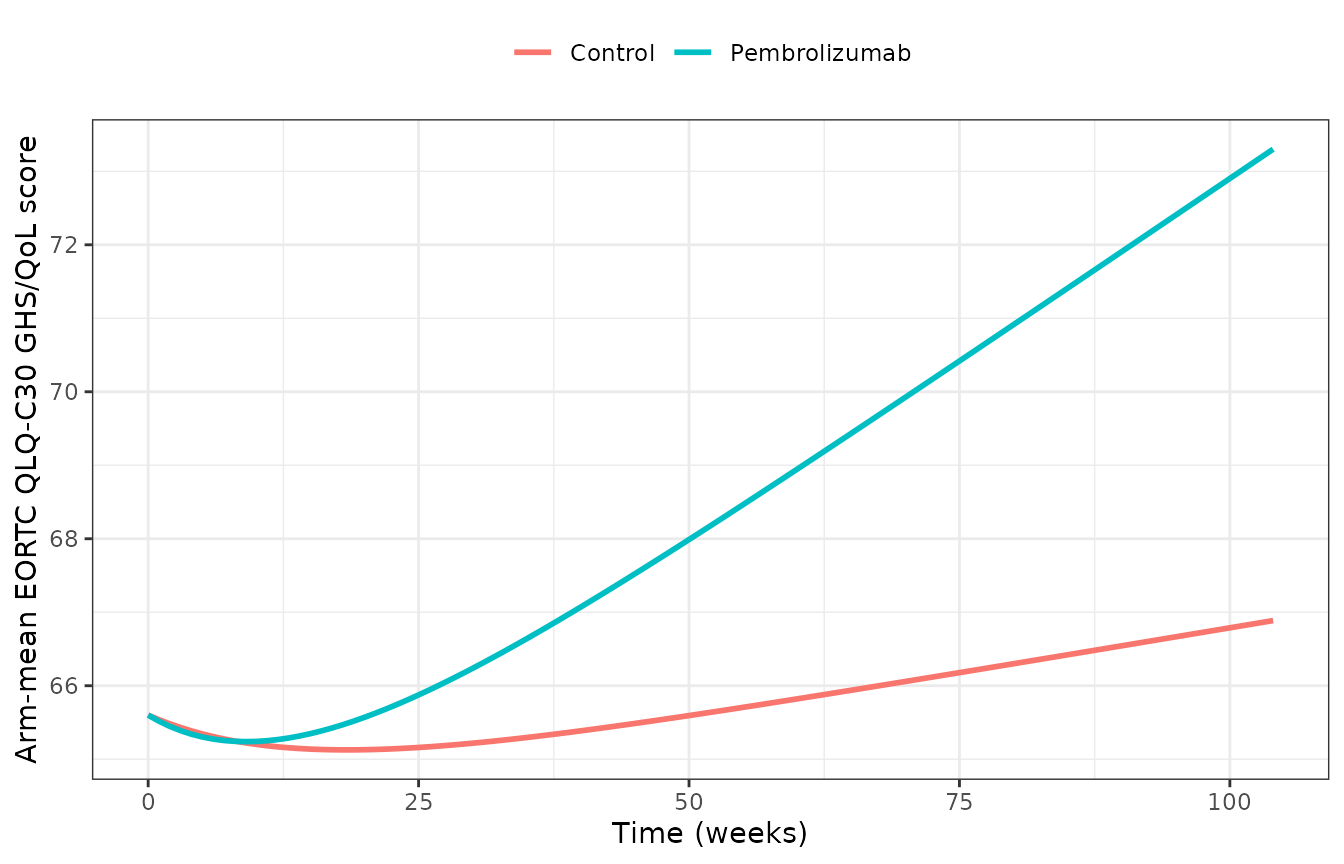
Replicates Figure 4A of Zou 2026: typical-value arm-mean QoL trajectories.
Nadir and long-term behaviour, quantified:
nadir <- tv_traj |>
  group_by(Arm) |>
  slice_min(qol_ghs, n = 1, with_ties = FALSE) |>
  ungroup() |>
  select(Arm, `Nadir week` = time, `Nadir score` = qol_ghs)
wk104 <- tv_traj |> filter(time == 104) |> select(Arm, `Week-104 score` = qol_ghs)
left_join(nadir, wk104, by = "Arm") |> knitr::kable(digits = 2)| Arm | Nadir week | Nadir score | Week-104 score |
|---|---|---|---|
| Control | 18 | 65.13 | 66.89 |
| Pembrolizumab | 9 | 65.24 | 73.30 |
pem_traj <- tv_traj |> filter(Arm == "Pembrolizumab") |> arrange(time)
ctl_traj <- tv_traj |> filter(Arm == "Control") |> arrange(time)
delta <- pem_traj$qol_ghs - ctl_traj$qol_ghs   # pembrolizumab minus control

stopifnot(
  identical(pem_traj$time, ctl_traj$time),
  # Both arms start at the same baseline: treatment acts on Emax and SLP only.
  abs(delta[pem_traj$time == 0]) < 1e-10,
  abs(pem_traj$qol_ghs[1] - 65.6) < 1e-8,
  # Early on, the larger pembrolizumab toxicity term dominates and the
  # pembrolizumab arm sits BELOW control.
  delta[pem_traj$time == 4] < 0,
  # A single crossover occurs, after which pembrolizumab stays above control
  # and the gap widens monotonically to the end of the simulated horizon.
  any(delta[pem_traj$time > 0] < 0), any(delta > 0),
  all(diff(delta[pem_traj$time >= 12]) > 0),
  tail(delta, 1) > 0
)
# Week at which pembrolizumab overtakes control.
pem_traj$time[which(delta > 0)[1]]
#> [1] 9
Simulated arm-level cohort
With both variability levels switched on, the spread across simulated arms is wide – which is the paper’s central methodological point: arm-level QoL data are so variable that a baseline-to-endpoint hypothesis test loses the signal that the longitudinal model recovers.
band <- closed |>
  mutate(Arm = ifelse(TRT == 0, "Pembrolizumab", "Control")) |>
  group_by(Arm, time) |>
  summarise(
    med = median(qol_ghs),
    lo  = quantile(qol_ghs, 0.1),
    hi  = quantile(qol_ghs, 0.9),
    .groups = "drop"
  )

ggplot(band, aes(time, med, colour = Arm, fill = Arm)) +
  geom_ribbon(aes(ymin = lo, ymax = hi), alpha = 0.15, colour = NA) +
  geom_line(linewidth = 1) +
  labs(x = "Time (weeks)", y = "Arm-mean EORTC QLQ-C30 GHS/QoL score", colour = NULL, fill = NULL) +
  theme_bw() +
  theme(legend.position = "top")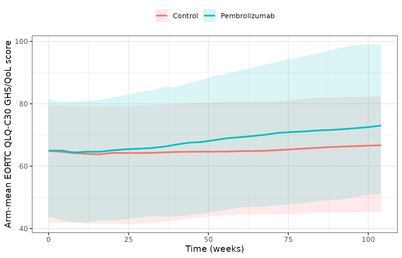
Simulated arm-mean QoL trajectories (200 arms per treatment group), median and 10th/90th percentiles.
The cohort-level assertion is deliberately made on the median
across arms, not on any extreme: the tails of a random cohort
are not reproducible across rxode2 versions, but the centre of a 200-arm
distribution is. Even the median carries sampling noise, so the bounds
below were set from measurement rather than from a single run – across
12 seeds the baseline median gap ranged -0.3 to +3.0 points (it is pure
noise; treatment does not act on E0 at all) and the
week-104 gap ranged +5.3 to +11.8 points. Each bound leaves at least
two-fold headroom over the observed range, so a different rxode2 RNG
stream cannot flip it.
med_wide <- band |>
  select(Arm, time, med) |>
  tidyr::pivot_wider(names_from = Arm, values_from = med)
base_gap  <- med_wide$Pembrolizumab[med_wide$time == 0] -
  med_wide$Control[med_wide$time == 0]
wk104_gap <- med_wide$Pembrolizumab[med_wide$time == 104] -
  med_wide$Control[med_wide$time == 104]

stopifnot(
  # Baseline medians agree to within cohort sampling noise: treatment acts on
  # Emax and SLP only, never on E0. (Observed |gap| <= 3.0 over 12 seeds.)
  abs(base_gap) < 6,
  # By week 104 the median pembrolizumab arm is clearly above the median
  # control arm. (Observed gap >= 5.3 over 12 seeds.)
  wk104_gap > 2
)
c(`baseline gap` = base_gap, `week-104 gap` = wk104_gap)
#> baseline gap week-104 gap
#>   -0.4271421    5.7336574
Assumptions and deviations
-
Saturation guard. Supplementary Codes section A
computes
Qsat = min(max(Q,0.01),0.99)with the comment “adding a saturation to avoid taking logit(0) (undefined)”, but its very next line takes the logit of the unsaturatedQ. This file takes the logit ofQsat, which is what the guard’s own comment says it is for. The deviation is a no-op over the typical-value trajectory and a necessity in a simulated cohort:Qis unbounded above, so a high-baseline, high-slope arm carries it past 1 at long times andlogit(Q)returnsNaN. In the 10,800-row cohort simulated above roughly 2% of rows are affected. The check below shows both facts.
# Typical values: the guard never binds, so the deviation changes nothing.
stopifnot(max(abs(tv_traj$qFrac - tv_traj$qSat)) == 0)

# Simulated cohort: the guard does bind. The clamped set is a SUPERSET of the
# rows that would have gone non-finite -- the guard's ceiling is 0.99, not 1,
# so it also catches the thin band where logit(Q) is finite but the arm mean
# would print above 99 on a 0-100 instrument.
n_clamped      <- sum(abs(closed$qFrac - closed$qSat) > 0)
n_would_be_nan <- sum(closed$qFrac <= 0 | closed$qFrac >= 1)
c(rows = nrow(closed), clamped = n_clamped, would_be_NaN = n_would_be_nan,
  max_qFrac = round(max(closed$qFrac), 3))
#>         rows      clamped would_be_NaN    max_qFrac
#>    10800.000      221.000      197.000        3.397

stopifnot(
  # The problem is real, not hypothetical: some arms do leave (0, 1).
  n_would_be_nan > 0,
  # Every row that would have gone non-finite is covered by the guard.
  n_would_be_nan <= n_clamped,
  # The guard binds only outside [0.01, 0.99], and never leaves it.
  all(abs(closed$qFrac - closed$qSat)[closed$qFrac >= 0.01 & closed$qFrac <= 0.99] == 0),
  all(closed$qSat >= 0.01), all(closed$qSat <= 0.99)
)
Observation scale. The paper’s dependent variable is
sqrt(N) * logit(y/100)(Eq. 2), fitted with a constant residual SDa(MonolixerrorModel=constant(a)). This file instead observeslogit(y/100)with residual SDa / sqrt(N), which is the same statement written as the article’s own Eq. 3 (eps ~ N(0, sigma^2 / N)). The two are algebraically identical; the Eq. 3 form is used so the observation stays on an interpretable scale and the arm-size weighting is visible inmodel().Random-effect naming.
checkModelConventions()warns thateta_study_e0,eta_study_emax,eta_arm_e0andeta_arm_slpdo not pair with fixed effects named_study_e0etc. The names are intentional: this is a two-level MBMA and theeta<param>convention cannot distinguish between-study variability from between-treatment-arm variability on the same parameter, which this model has onE0. Theeta_study_*form follows the existing library precedent inMercier_2014_tramadol_tapentadol_mbmaandChen_2025_methotrexate_das28_mbma.Not an exposure-response model. No pembrolizumab dose or concentration enters the model. Pembrolizumab monotherapy and pembrolizumab-combination arms are pooled into a single
TRT = 0level, and every comparator regimen (chemotherapy, targeted therapy, placebo plus standard of care, placebo alone) is pooled intoTRT = 1. The model therefore cannot answer dose-optimisation questions, and a “control” effect here is an average over heterogeneous comparators.Covariates screened but not retained. Age, the arm’s male proportion, the arm’s ECOG-0 proportion, the arm’s stage IV proportion and tumour type were all screened by the full fixed-effects covariate model (Section 2.5) and none was retained (Section 3.2). They are recorded in the model file’s
covariatesDataExcludedmetadata so the provenance of the screen survives. The paper is explicit that the tumour-type null is a power limitation rather than evidence of no effect: “the dataset lacked sufficient power to compare pembrolizumab’s QoL benefits across different tumor types” (Limitations). No point estimate is published for any screened covariate, so none can be encoded even optionally.No PKNCA section. NCA is not meaningful for this model: there is no drug concentration, no dose and no ODE state. The closed-form, weighting, bounded-score and treatment-effect gates above take its place, following the package’s validation pattern for models where PKNCA is not the right check.
n_subjectsis derived, not published. The paper reports 410 observations (228 pembrolizumab, 182 control) but no participant total. Thepopulation$n_subjectsvalue of 11326 is a lower bound: the sum of the Table 1 baseline arm sizes (12345) minus the 1019 participants of the second KEYNOTE-054 (NCT02362594) row, which appears twice (Bottomley 2021 and Buhrer 2024). Table 1 footnote a notes the two entries “were published with different population inclusion criteria and follow-up durations”, so they overlap heavily without being the identical cohort, and the exact unique count cannot be recovered from what is published.Informative dropout is not modelled. The paper’s own Limitations paragraph notes that QoL assessments after treatment discontinuation were typically missing and not imputed, so arm-level trajectories may over-represent patients with favourable outcomes at later timepoints and the long-term QoL benefit may be overestimated. Simulations at long times inherit that bias.