Nusinersen (Biliouris 2018)
Source:vignettes/articles/Biliouris_2018_nusinersen.Rmd
Biliouris_2018_nusinersen.RmdModel and source
- Citation: Biliouris K, Gaitonde P, Yin W, Norris DA, Wang Y, Henry S, Fey R, Nestorov I, Schmidt S, Rogge M, Lesko LJ, Trame MN. A Semi-Mechanistic Population Pharmacokinetic Model of Nusinersen: An Antisense Oligonucleotide for the Treatment of Spinal Muscular Atrophy. CPT Pharmacometrics Syst Pharmacol. 2018;7(9):581-592. doi:10.1002/psp4.12323
- Description: Semimechanistic nine-compartment population PK model of nusinersen (antisense oligonucleotide, Biogen ISIS 396443) intended for extrapolation of nonhuman-primate (cynomolgus monkey) fits to paediatric patients with spinal muscular atrophy, following intrathecal lumbar-puncture bolus administration. Structure (Biliouris 2018): CSF is the sampled dosing site, coupled bidirectionally to three anatomically distinct spinal-cord segments (cervical, thoracic, lumbar), to the brain (with a deeper brain-tissue redistribution compartment), and to the pons; CSF also drains one-way into the plasma / central compartment, which has its own peripheral distribution and first-order elimination. Volumes scale linearly with body weight relative to a 2.8 kg reference; rate constants scale as (WT/2.8)^(-0.08); the CSF physiological volume V_CSF is overridden by a stepwise paediatric-age function (120, 130, 135, 140 mL for age classes <0.25, 0.25-0.5, 0.5-1, 1-2 years) rather than by WT. Residual error is proportional per observed matrix; twelve exponential-IIV terms are carried on the elimination and transfer rate constants and on the CSF / plasma volumes. All THETA / OMEGA / SIGMA values are held FIXED from the paper’s final NONMEM simulation control stream on file.
- Article: https://doi.org/10.1002/psp4.12323
The available source is the paper’s simulation NONMEM control stream
($PROBLEM SMA MONKEY,
$SIMULATION (12345678) ONLYSIM SUBPROBLEM=1000). All
$THETA, $OMEGA, and $SIGMA
entries carry the FIX flag, so every value in the packaged
ini() block is wrapped in fixed(). See
“Assumptions and deviations” below for the paper-text sections not
available with the control stream.
Population
The Biliouris 2018 model was originally fitted to cynomolgus-monkey
plasma and CNS-tissue data (the $PROBLEM tag “SMA MONKEY”
identifies the fit dataset). The simulation control stream then re-uses
the monkey-fit parameter estimates for a paediatric-human extrapolation:
volumes are linearly weight-scaled from a 2.8 kg reference, rate
constants use a slight (WT/2.8)^(-0.08) scaling, and the
CSF physiological volume V_CSF is overridden by a stepwise
age function that matches human paediatric CSF anatomy (120, 130, 135,
140 mL for age classes < 0.25, 0.25 to < 0.5, 0.5 to < 1, 1 to
< 2 years; adult reference 150 mL). Full baseline demographics for
the fitted monkey cohort are not included with the supplementary
simulation stream; refer to Biliouris 2018 main text Methods and Table 1
(published in CPT Pharmacometrics Syst Pharmacol) for
n_subjects, age, and sex distributions.
The population metadata packaged with the model is available programmatically:
mod_fun <- readModelDb("Biliouris_2018_nusinersen")
str(mod_fun()$population, max.level = 1)
#> List of 10
#>  $ species              : chr "cynomolgus monkey (juvenile) with paediatric-human physiological scaling"
#>  $ n_subjects           : logi NA
#>  $ n_studies            : logi NA
#>  $ age_range            : chr "monkey fit + paediatric-human simulation window of 0-2 years for the V_CSF table"
#>  $ weight_range         : chr "reference body weight 2.8 kg (monkey / newborn-scale)"
#>  $ disease_state        : chr "Spinal muscular atrophy (SMA) target indication; monkey $PROBLEM tag 'SMA MONKEY'"
#>  $ dose_range           : chr "Intrathecal lumbar-puncture bolus (simulated at 1-12 mg per paediatric-clinic protocol)"
#>  $ administration_routes: chr "Intrathecal bolus into CSF"
#>  $ regions              : chr "Preclinical / translational (cynomolgus-monkey fit extrapolated to paediatric SMA patients)"
#>  $ notes                : chr "The source for this model is the paper's simulation NONMEM control stream (`$PROBLEM SMA MONKEY`, `$SIMULATION "| __truncated__
Source trace
Every value below is traced to the paper’s simulation NONMEM control
stream (a five-page PDF containing the $PROBLEM SMA MONKEY
model verbatim). The full $THETA(k) FIX /
$OMEGA k FIX label is repeated as the in-file comment on
each ini() entry.
| Structural element | Value | Source location |
|---|---|---|
V1 = 150 mL (CSF adult) |
lv_csf = fixed(log(150)) |
$THETA(1) 150 FIX ; (1. V1) mL |
V2 = 937 mL (plasma) |
lv_plasma = fixed(log(937)) |
$THETA(2) 937 FIX ; (2. V2) mL |
V3 = 1.91 mL (cervical SC) |
lv_cerv = fixed(log(1.91)) |
$THETA(3) 1.91 FIX ; (3. V3) mL |
V4 = 53.8 mL (brain) |
lv_brain = fixed(log(53.8)) |
$THETA(4) 53.8 FIX ; (4. V4) mL |
V6 = 1.08 mL (lumbar SC) |
lv_lumb = fixed(log(1.08)) |
$THETA(20) 1.08 FIX ; (20. V6) mL |
V8 = 1.52 mL (thoracic SC) |
lv_thor = fixed(log(1.52)) |
$THETA(25) 1.52 FIX ; (25. V8) mL |
V9 = 2.11 mL (pons) |
lv_pons = fixed(log(2.11)) |
$THETA(28) 2.11 FIX ; (28. V9) mL |
K12 = 0.0891 1/h (CSF -> plasma) |
lk_csf_plasma |
$THETA(9) 0.0891 FIX ; (9. K12) |
K20 = 0.206 1/h (plasma elim) |
lkel |
$THETA(10) 0.206 FIX ; (10. K20) |
K13/K31, K14/K41, K25/K52, K16/K61, K47/K74, K18/K81, K19/K91 |
all fixed(log(...))
|
$THETA(5..8, 11..12, 21..24, 26..27, 29..30) |
V1(AGE) overrides: 120/130/135/140 mL for AGE < 0.25
/ < 0.5 / < 1 / < 2 y |
in model() ifelse chain |
$PK IF (AGE.LT.0.25) TVV1 = 120 etc. |
Volume WT scaling: V = TVV * (WT/2.8) for
V2..V9 (not V1) |
wt_ratio = WT/2.8 in model()
|
$PK TVV_i = THETA(_i) * (WT/2.8); V1’s
(WT/2.8) is commented out |
Rate WT scaling:
K = TVK * (WT/2.8)^(-0.08)
|
wt_kfac = wt_ratio^e_wt_k |
$PK TVK_ij = THETA(_) * 1/((WT/2.8)**0.08) |
| Twelve exponential IIVs on K20, K12, V1, V2, K13, K14, K41, K16, K18, K81, K19, K91 |
~ fixed(<var>) diagonal |
$OMEGA variances 0.421, 1.3, 0.854, 0.832, 0.453, 13.6,
0.153, 0.124, 0.28, 0.129, 0.654, 0.289 (all FIX) |
| Proportional residual SD per tissue |
propSd_Ccsf = 0.714, propSd = 0.412,
propSd_Ccerv = 0.101, propSd_Cbrain = 1.77,
propSd_Clumb = 0.312, propSd_Cthor = 0.0239,
propSd_Cpons = 0.0103 |
$THETA(13..19) FIX ; ERR1..ERR9;
$SIGMA 1 FIX combined with
W = SQRT(THETA^2 * IPRED^2) makes THETA the
SD-fraction |
The nine ODEs replicate the paper’s $DES block
one-for-one; the in-line comments in
inst/modeldb/specificDrugs/Biliouris_2018_nusinersen.R give
the paper-to-model mapping compartment-by-compartment.
Virtual cohort
The paper does not provide observed data. The figures below use two paediatric-focused virtual populations for a single 12 mg intrathecal lumbar-puncture bolus (the fixed dose used in the ISIS 396443 clinical programme).
Cohort 1 (typical-value trajectories): one
representative five-year-old (15 kg, AGE 5 y). All random effects
zeroed. V_CSF = 150 mL (adult regime).
Cohort 2 (pediatric VPC): 100 virtual paediatric
subjects with weight uniformly in 5 to 20 kg and age uniformly in 0.1 to
2 y. The age range exercises the V_CSF step function (each
of the four paediatric bins is sampled).
set.seed(20260709)

obs_grid <- c(0, 0.5, 1, 2, 4, 8, 12, 24, 36, 48, 72, 96, 120, 144, 168)

# Cohort 1 -- single-subject typical trajectories
cohort1_events <- {
  dose <- data.frame(id = 1L, time = 0, amt = 12, cmt = "csf",
                     evid = 1L, dvid = NA_integer_,
                     WT = 15, AGE = 5, cohort = "typical (15 kg, 5 y)",
                     stringsAsFactors = FALSE)
  obs <- expand.grid(id = 1L, time = obs_grid,
                     dvid = 1:7, stringsAsFactors = FALSE)
  obs$amt   <- NA_real_
  obs$cmt   <- c("Ccsf", "Cc", "Ccerv", "Cbrain",
                 "Clumb", "Cthor", "Cpons")[obs$dvid]
  obs$evid  <- 0L
  obs$WT    <- 15
  obs$AGE   <- 5
  obs$cohort <- "typical (15 kg, 5 y)"
  rbind(dose, obs)
}

# Cohort 2 -- 100-subject paediatric VPC
n_ped <- 100L
cohort2_events <- {
  ped_wt  <- runif(n_ped, 5, 20)
  ped_age <- runif(n_ped, 0.1, 2)
  dose_rows <- data.frame(
    id    = seq_len(n_ped) + 100L,
    time  = 0,
    amt   = 12,
    cmt   = "csf",
    evid  = 1L,
    dvid  = NA_integer_,
    WT    = ped_wt,
    AGE   = ped_age,
    cohort = "paediatric VPC (5-20 kg, 0.1-2 y)",
    stringsAsFactors = FALSE
  )
  obs_rows <- do.call(rbind, lapply(seq_len(n_ped), function(i) {
    o <- expand.grid(id = 100L + i, time = obs_grid,
                     dvid = c(1L, 2L),  # Ccsf and Cc only, to keep the run light
                     stringsAsFactors = FALSE)
    o$amt   <- NA_real_
    o$cmt   <- c("Ccsf", "Cc")[o$dvid]
    o$evid  <- 0L
    o$WT    <- ped_wt[i]
    o$AGE   <- ped_age[i]
    o$cohort <- "paediatric VPC (5-20 kg, 0.1-2 y)"
    o
  }))
  rbind(dose_rows, obs_rows)
}

events <- rbind(cohort1_events, cohort2_events)
stopifnot(!anyDuplicated(unique(events[, c("id", "time", "evid", "dvid")])))
Simulation
mod <- readModelDb("Biliouris_2018_nusinersen")
sim <- rxode2::rxSolve(mod, events = events,
                       keep = c("WT", "AGE", "cohort", "dvid"))
#> ℹ parameter labels from comments will be replaced by 'label()'
sim_df <- as.data.frame(sim)
Typical-value trajectories (Cohort 1) use the zero-random-effect package model to replicate the paper’s semi-mechanistic prediction. VPC percentiles (Cohort 2) apply the paper’s fixed OMEGA variances.
mod_typ <- rxode2::zeroRe(mod)
#> ℹ parameter labels from comments will be replaced by 'label()'
sim_typ_df <- as.data.frame(
  rxode2::rxSolve(mod_typ, events = cohort1_events,
                  keep = c("WT", "AGE", "cohort"))
)
#> ℹ omega/sigma items treated as zero: 'etalkel', 'etalk_csf_plasma', 'etalv_csf', 'etalv_plasma', 'etalk_csf_cerv', 'etalk_csf_brain', 'etalk_brain_csf', 'etalk_csf_lumb', 'etalk_csf_thor', 'etalk_thor_csf', 'etalk_csf_pons', 'etalk_pons_csf'
Typical-value time course across sampled tissues
The seven ~ prop() residual-error clauses correspond to
the seven sampled matrices in the paper’s $ERROR block:
CSF, plasma, cervical spinal cord, brain, lumbar spinal cord, thoracic
spinal cord, and pons. Each panel below traces its algebraic observable
(Ccsf, Cc, Ccerv,
Cbrain, Clumb, Cthor,
Cpons) over 7 days after a single 12 mg intrathecal bolus
in the typical 15 kg / 5 y subject.
tissue_labels <- c(
  Ccsf   = "CSF",
  Cc     = "Plasma",
  Ccerv  = "Cervical spinal cord",
  Cbrain = "Brain",
  Clumb  = "Lumbar spinal cord",
  Cthor  = "Thoracic spinal cord",
  Cpons  = "Pons"
)

sim_typ_long <- sim_typ_df |>
  dplyr::select(time, dplyr::all_of(names(tissue_labels))) |>
  tidyr::pivot_longer(-time, names_to = "obs", values_to = "conc") |>
  dplyr::mutate(tissue = factor(tissue_labels[obs],
                               levels = unname(tissue_labels)))

ggplot(sim_typ_long, aes(time, pmax(conc, 1e-3))) +
  geom_line() +
  facet_wrap(~tissue, scales = "free_y") +
  scale_y_log10() +
  labs(x = "Time after 12 mg IT bolus (h)",
       y = "Concentration (ng/mL)",
       title = "Typical-value concentrations across the seven sampled matrices",
       caption = paste0("Semi-mechanistic 9-compartment nusinersen model ",
                        "(Biliouris 2018); zero random effects; ",
                        "typical 15 kg, 5 y subject."))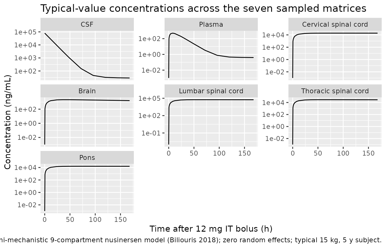
Virtual paediatric VPC on CSF and plasma
CSF (dose site) and plasma (systemic) are the two matrices where the paper’s model is most directly informative for clinical dosing.
vpc_df <- sim_df |>
  dplyr::filter(cohort == "paediatric VPC (5-20 kg, 0.1-2 y)") |>
  dplyr::select(id, time, WT, AGE, dvid, Ccsf, Cc) |>
  dplyr::mutate(matrix = c("CSF (ng/mL)", "Plasma (ng/mL)")[dvid],
                conc   = ifelse(dvid == 1L, Ccsf, Cc)) |>
  dplyr::filter(!is.na(conc), conc > 0)

vpc_summary <- vpc_df |>
  dplyr::group_by(matrix, time) |>
  dplyr::summarise(
    Q05 = quantile(conc, 0.05, na.rm = TRUE),
    Q50 = quantile(conc, 0.50, na.rm = TRUE),
    Q95 = quantile(conc, 0.95, na.rm = TRUE),
    .groups = "drop"
  )

ggplot(vpc_summary, aes(time, Q50)) +
  geom_ribbon(aes(ymin = Q05, ymax = Q95), alpha = 0.25) +
  geom_line() +
  facet_wrap(~matrix, scales = "free_y") +
  scale_y_log10() +
  labs(x = "Time after 12 mg IT bolus (h)",
       y = "Concentration (ng/mL)",
       title = "Paediatric VPC (n = 100, 5-20 kg, 0.1-2 y): CSF + plasma",
       caption = "5th, 50th, 95th percentiles of virtual subjects.")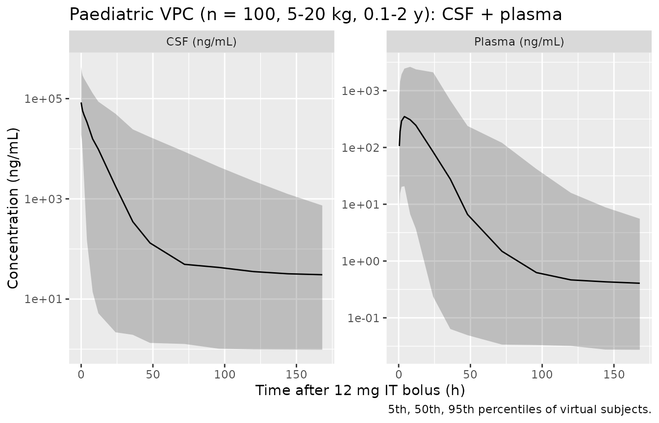
PKNCA on typical-value plasma exposure
The paper does not tabulate NCA parameters for the semi-mechanistic extrapolation, so the block below serves as a sanity summary rather than a validation-table comparison: it confirms that the packaged model reproduces plausible plasma Cmax, Tmax, terminal half-life, and AUC after a single 12 mg IT dose in the typical paediatric subject.
# rxSolve drops the id column for single-subject sims; add it back so
# PKNCA gets a per-subject key.
if (!"id" %in% names(sim_typ_df)) sim_typ_df$id <- 1L

pk_conc <- sim_typ_df |>
  dplyr::select(id = id, time = time, Cc = Cc, cohort = cohort) |>
  dplyr::filter(!is.na(Cc))

# Time-zero guarantee -- PKNCA needs a time = 0 row per (id, cohort).
pk_conc <- dplyr::bind_rows(
  pk_conc,
  pk_conc |> dplyr::distinct(id, cohort) |>
    dplyr::mutate(time = 0, Cc = 0)
) |>
  dplyr::distinct(id, cohort, time, .keep_all = TRUE) |>
  dplyr::arrange(id, cohort, time)

conc_obj <- PKNCA::PKNCAconc(pk_conc, Cc ~ time | cohort + id)

dose_df <- cohort1_events |>
  dplyr::filter(evid == 1L) |>
  dplyr::select(id, time, amt, cohort)
dose_obj <- PKNCA::PKNCAdose(dose_df, amt ~ time | cohort + id)

intervals <- data.frame(
  start = 0, end = Inf,
  cmax = TRUE, tmax = TRUE, aucinf.obs = TRUE, half.life = TRUE
)

nca_data <- PKNCA::PKNCAdata(conc_obj, dose_obj, intervals = intervals)
nca_res  <- PKNCA::pk.nca(nca_data)

nca_res$result |>
  dplyr::select(cohort, PPTESTCD, PPORRES) |>
  tidyr::pivot_wider(names_from = PPTESTCD, values_from = PPORRES) |>
  dplyr::rename(
    "Cohort"                       = cohort,
    "Cmax (ng/mL)"                 = cmax,
    "Tmax (h)"                     = tmax,
    "AUC[0,inf] observed (ng.h/mL)" = aucinf.obs,
    "t1/2 (h)"                     = half.life
  ) |>
  knitr::kable(digits = 3,
caption = "Plasma NCA on the typical-value replication (n = 1).")| Cohort | Cmax (ng/mL) | Tmax (h) | tlast | clast.obs | lambda.z | r.squared | adj.r.squared | lambda.z.time.first | lambda.z.time.last | lambda.z.n.points | clast.pred | t1/2 (h) | span.ratio | AUC[0,inf] observed (ng.h/mL) |
|---|---|---|---|---|---|---|---|---|---|---|---|---|---|---|
| typical (15 kg, 5 y) | 503.188 | 8 | 168 | 0.399 | 0.048 | 0.888 | 0.871 | 12 | 168 | 9 | 0.096 | 14.314 | 10.899 | 10837.99 |
Assumptions and deviations
-
The available source is the simulation control stream, not
the full paper text. The five-page PDF contains only the
$PROBLEM SMA MONKEYsimulation model ($SIMULATION (12345678) ONLYSIM SUBPROBLEM=1000) with every$THETA,$OMEGA, and$SIGMAvalue carrying theFIXflag. All packaged values are traced verbatim to that block. Baseline demographics for the fitted monkey cohort, the paper’s narrative Methods, and any published NCA comparison values live in Biliouris 2018 main text (CPT PSP 2018;7(9):581-592) and are not reproduced here. -
V_CSFpiecewise age function is a paediatric-human anatomical overlay. The paper’s$PKblock replaces the fitted V1 = 150 mL with anatomically scaled paediatric values viaIF (AGE.LT.0.25) TVV1 = 120etc. TheWTscaling term(WT/2.8)is explicitly commented out for V1 in the control stream, soV_CSFis set by the age function alone. -
Reference weight 2.8 kg (newborn / juvenile-scale)
is coded verbatim from the
$PKblock’s(WT/2.8)factor. Applied linearly to V2..V9 and as(WT/2.8)^(-0.08)to every rate constant, per the simulation-file description (“scale exp -0.08”). -
Twelve exponential IIVs, twelve diagonal
$OMEGAvariances. The paper’s$PKblock explicitly comments out ETA on K31, K25, K52, V3, V4, V6, K61, K47, K74, V8, V9, so those individual parameters are typical-value only. Theetalk_csf_brain ~ fixed(13.6)variance is unusually large (log-scale variance 13.6 implies a CV so large that stochastic VPCs on K14 will explode) and is retained verbatim from the paper’s$OMEGAblock; users running stochastic VPCs should be aware. -
Residual error interpretation. The paper’s
$ERRORblock isW = SQRT(THETA(k)^2 * IPRED^2)andY = IPRED + W * ERR(1)with$SIGMA 1 FIX, soW = |THETA(k)| * |IPRED|andTHETA(k)is the proportional-SD fraction on the linear (untransformed) scale. That is whatpropSd_<output>records. -
Bioavailability scaling. The dose is in mg but
volumes are in mL, so
f(csf) <- 1e6converts each dose to ng in the state and the observations come out directly in ng/mL. No paper-side conversion is implied. -
Compartment naming. Cervical, lumbar, and thoracic
spinal-cord compartments and the pons compartment are declared as
paper_specific_compartments(they do not have canonical entries in thebrain_<region>/spinal_cord_<segment>families as of this writing). Plasma is mapped to the canonicalcentral, matching the Luu 2017 nusinersen model.