Mitoxantrone PBPK with DNA + macromolecule binding (An 2012)
Source:vignettes/articles/An_2012_mitoxantrone_pbpk.Rmd
An_2012_mitoxantrone_pbpk.RmdModel and source
- Citation: An G, Morris ME. A Physiologically Based Pharmacokinetic Model of Mitoxantrone in Mice and Scale-up to Humans: a Semi-Mechanistic Model Incorporating DNA and Protein Binding. AAPS J. 2012;14(2):352-364.
- Article: https://doi.org/10.1208/s12248-012-9344-7
Mitoxantrone (Novantrone) is a synthetic anthracenedione anticancer agent with high efficacy in breast cancer, acute leukemia, non-Hodgkin’s lymphoma and secondary progressive multiple sclerosis. Its cytotoxicity is mediated through DNA intercalation; mitoxantrone also binds microsomal protein in tissue. An and Morris (2012) reported the first mechanism-based PBPK model for mitoxantrone, evaluating three candidate structures (Model 1: classical Kp values, Model 2: deep binding compartment, Model 3: explicit DNA + macromolecule binding) and selecting Model 3 as the only one that captured both plasma and tissue data well. Model 3 is the implementation packaged in nlmixr2lib; Models 1 and 2 are not packaged because the authors rejected them in favor of Model 3 (paper Results section).
The mouse PBPK fit anchors the binding constants (K_DNA,
K_macro) and the tissue protein-binding capacities
(T_macro). The human-scaled simulation re-uses those
mouse-fit constants under the paper’s cross- mammalian assumption
(“Blood and tissue distribution parameters, including fu (0.2), K_DNA
(0.0013 uM), K_macro (1.44 uM), and T_macro in different tissues … were
assumed to be identical in mammals”) and substitutes human DNA contents
from the literature (Gustafson 2002, Methods text) for the tissue T_DNA
values.
Population
Mouse cohort
- Male ND4 Swiss Webster mice (Harlan Labs), 24-32 g (mean 27.4 g), housed at 12 h light / 12 h dark with standard diet and water ad libitum.
- Single 5 mg/kg IV bolus via penile vein.
- Destructive sampling at 5, 15, 30 min and 1, 2, 4, 8, 48 h with 3-4 animals per time point.
- Plasma + six tissues (lung, heart, spleen, liver, kidney, brain) assayed by validated HPLC (LLOQ plasma 5 ng/mL, tissue homogenate 12.5 ng/mL).
Human cohort
The An and Morris 2012 human simulation is a pure forward projection against the digitised plasma concentration vs. time data from two previously published clinical pharmacokinetic studies after a 12 mg/m^2 IV bolus of mitoxantrone:
- Larson et al. 1987 J Clin Oncol 5:391-7 (acute non-lymphocytic leukemia).
- Peng et al. 1982 J Chromatogr 233:235-47 (advanced breast cancer).
No individual-level data were fit; the human PBPK model is a typical- value forward projection.
The full metadata for either species is available programmatically
via the model’s population slot
(readModelDb("An_2012_mitoxantrone_mouse_pbpk")$population
or
readModelDb("An_2012_mitoxantrone_human_pbpk")$population).
Source trace
The per-parameter origin is recorded as an in-file comment next to
each ini() entry in
inst/modeldb/specificDrugs/An_2012_mitoxantrone_mouse_pbpk.R
and
inst/modeldb/specificDrugs/An_2012_mitoxantrone_human_pbpk.R.
The table below collects them for review.
| Quantity | Mouse value | Human value | Source location |
|---|---|---|---|
| Eq 9 (well-stirred tissue ODE with binding Kp_eff(Cp)) | derivation | derivation | Methods, p.356 |
| Eq 10-11 (permeability-limited remainder, ISF + intracellular) | derivation | derivation | Methods, p.356 |
| Eq 1 (organ blood flow scaling Q2 = BW2 * Q1 / BW1) | derivation | not used | Methods, p.355 |
| Eq 13 (PS allometric scaling PS = A * M^0.75) | not used | derivation | Methods, p.357 |
| Eq 14 (well-stirred rearrangement for Clint from CL) | not used | derivation | Methods, p.357 |
| fu (unbound fraction in plasma) | 0.2 (fixed) | 0.2 (fixed) | Data Analysis, p.357 |
| K_DNA (uM) | 0.0013 (RSE 29%) | 0.0013 (inherited) | Table II Model 3 |
| K_macro (uM) | 1.44 (RSE 52%) | 1.44 (inherited) | Table II Model 3 |
| T_DNA lung (uM) | 16.2 (RSE 13%) | 15 | mouse Table II / human Table III |
| T_DNA heart (uM) | 20.6 (fixed) | 8.3 | mouse Table I / human Table III |
| T_DNA spleen (uM) | 18.4 (RSE 18%) | 15 | mouse Table II / human Table III |
| T_DNA liver (uM) | 26.0 (fixed) | 23.7 | mouse Table I / human Table III |
| T_DNA kidney (uM) | 50.2 (fixed) | 16.2 | mouse Table I / human Table III |
| T_DNA brain (uM) | 0.10 (RSE 11%) | 0.10 (mouse-derived) | mouse Table II / Table III footnote d |
| T_DNA remainder (uM) | 4.82 (RSE 43%) | 4.5 | mouse Table II / human Table III |
| T_macro lung (uM) | 19.0 (RSE 87%) | 19 (inherited) | Table II Model 3 |
| T_macro heart (uM) | 43.8 (fixed) | 43.8 (inherited) | Table I / Table III |
| T_macro spleen (uM) | 3.54 (RSE >300%) | 3.54 (inherited) | Table II Model 3 |
| T_macro liver (uM) | 514 (RSE 45%) | 514 (inherited) | Table II Model 3 |
| T_macro kidney (uM) | 52.3 (fixed) | 52.3 (inherited) | Table I / Table III |
| T_macro brain | implicit 0 | implicit 0 | Table I / Table III (entry “-”) |
| T_macro remainder (uM) | 4.67 (RSE >300%) | 4.67 (inherited) | Table II Model 3 |
| Clint_H | 29.5 mL/min = 1.77 L/h | 250 L/h | Results paragraph / Methods text |
| Clint_R | 2.14 mL/min = 0.128 L/h | 27 L/h | Results paragraph / Methods text |
| PS_remainder | 1.44 mL/min = 0.0864 L/h | 31.1 L/h | Results paragraph / Methods text |
| Q_i (organ blood flows) | Table I col “model 3” | Table III col “Blood flow rate” | Tables I / III |
| V_i (organ volumes) | Table I col “model 3” | Table III col “Organ volume” | Tables I / III |
| V_ISF, V_int (remainder) | Table I (8.26, 16.77 mL) | mouse 33/67 split applied to V_other = 62 L | Table I (mouse) / vignette Assumptions (human) |
| Mitoxantrone MW (g/mol) | 444.49 | 444.49 | DrugBank DB01204 / PubChem CID 4212 |
| sigma1, sigma2 (residual error) | not reported | not reported | placeholder propSd = 0.10 (see Assumptions) |
Units in the ODE system
| Quantity | Units |
|---|---|
| Time | hour |
| Volumes (mouse) | L (Table I mL / 1000) |
| Volumes (human) | L (Table III L) |
| Organ blood flows Q_i | L/h (mouse Table I mL/min * 60/1000; human Table III L/min * 60) |
| Clint_H, Clint_R, PS | L/h |
| Amounts (state values) | mg |
| Concentrations (state / volume) | mg/L (= ug/mL = ng/mL * 1e-3) |
| T_DNA, T_macro, K_DNA, K_macro | uM (paper notation; nmol/g for T_DNA / T_macro in Table II equates to uM under 1 g tissue ~ 1 mL assumption) |
| fu | unitless |
| Mitoxantrone molecular weight | 444.49 g/mol |
| Body weight (covariate WT, mouse) | kg (5 mg/kg * WT for IV dose mass) |
| Body surface area (covariate BSA, human) | m^2 (12 mg/m^2 * BSA for IV dose mass) |
Doses are supplied in mg. For the mouse model, a 5 mg/kg dose in a
27.4 g animal is 5 * 0.0274 = 0.137 mg; for the human
model, a 12 mg/m^2 dose in a 1.73 m^2 adult is
12 * 1.73 = 20.76 mg.
Mouse simulation
mod_mouse <- readModelDb("An_2012_mitoxantrone_mouse_pbpk")
mod_mouse_typical <- rxode2::zeroRe(mod_mouse)
#> Warning: No omega parameters in the model

# 5 mg/kg in a 27.4 g mouse -> 0.137 mg IV bolus.
bw_mouse <- 0.0274
dose_mouse_mg <- 5 * bw_mouse

events_mouse <- rxode2::et(amt = dose_mouse_mg, cmt = "central", time = 0) |>
  rxode2::et(time = c(0, 1/12, 0.25, 0.5, 1, 2, 4, 8, 16, 24, 36, 48)) |>
  as.data.frame() |>
  dplyr::mutate(id = 1L, treatment = "IV 5 mg/kg", WT = bw_mouse)

sim_mouse <- rxode2::rxSolve(
  mod_mouse_typical, events = events_mouse,
  keep = c("treatment", "WT", "id")
) |> as.data.frame() |>
  dplyr::mutate(id = 1L)
#> Warning: 'keep' contains id
#> which are output when needed, ignoring these items
Replicate Figure 5c (mouse, Model 3): tissue concentration-time profiles
The plot below renders the typical-value Model 3 prediction for plasma and the six measured tissues after the IV 5 mg/kg dose in the mean 27.4 g mouse. The y-axis is log-scaled mg/L (= ug/mL); the original Figure 5c uses log ug/mL with overlaid 3-4-mouse mean +/- SD HPLC observations.
mouse_long <- sim_mouse |>
  dplyr::filter(time > 0, time <= 48) |>
  dplyr::transmute(
    time,
    Plasma = Cc,
    Lung   = c_lung,
    Heart  = c_heart,
    Spleen = c_spleen,
    Liver  = c_liver,
    Kidney = c_kidney,
    Brain  = c_brain
  ) |>
  tidyr::pivot_longer(-time, names_to = "tissue", values_to = "conc")

ggplot(mouse_long, aes(time, conc)) +
  geom_line() +
  facet_wrap(~tissue, ncol = 3, scales = "free_y") +
  scale_y_log10() +
  labs(x = "Time (h)", y = "Mitoxantrone concentration (mg/L)",
       title = "Mouse Model 3: plasma and tissue concentration-time profiles",
       caption = "Replicates Figure 5c of An and Morris 2012 (typical-value prediction).")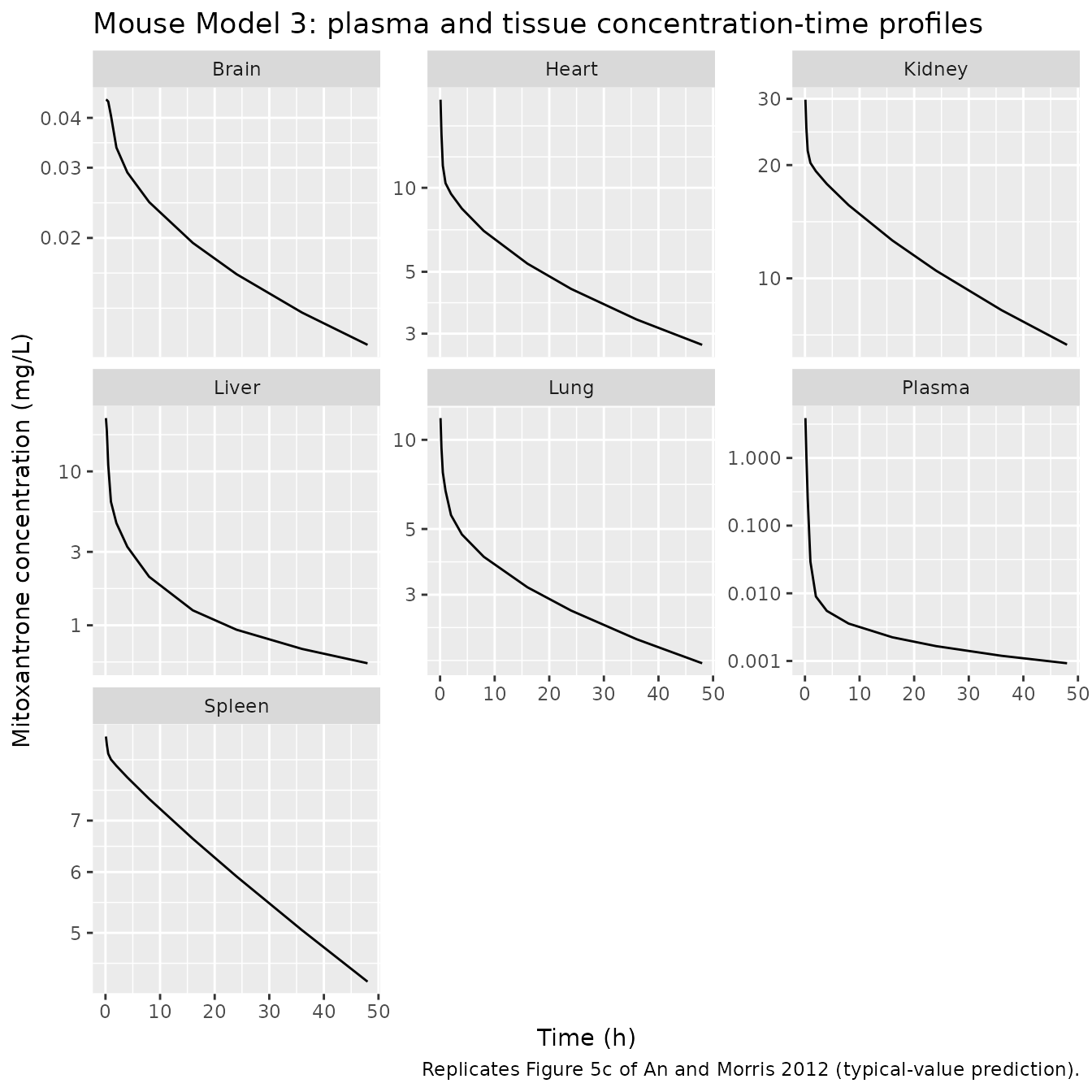
PKNCA validation (mouse plasma)
mouse_dense <- rxode2::et(amt = dose_mouse_mg, cmt = "central", time = 0) |>
  rxode2::et(time = c(0, seq(1/60, 48, by = 0.1))) |>
  as.data.frame() |>
  dplyr::mutate(id = 1L, treatment = "IV 5 mg/kg", WT = bw_mouse)
sim_dense <- rxode2::rxSolve(mod_mouse_typical, events = mouse_dense,
                             keep = c("treatment", "WT", "id")) |>
  as.data.frame() |>
  dplyr::mutate(id = 1L)
#> Warning: 'keep' contains id
#> which are output when needed, ignoring these items

nca_conc <- sim_dense |>
  dplyr::filter(time > 0, !is.na(Cc)) |>
  dplyr::select(id, time, Cc, treatment)

dose_df <- mouse_dense |>
  dplyr::filter(evid == 1) |>
  dplyr::transmute(id, time, amt, treatment)

conc_obj <- PKNCA::PKNCAconc(nca_conc, Cc ~ time | treatment + id,
                             concu = "mg/L", timeu = "h")
dose_obj <- PKNCA::PKNCAdose(dose_df, amt ~ time | treatment + id,
                             doseu = "mg")

mouse_intervals <- data.frame(
  start = 0, end = 48,
  cmax = TRUE, tmax = TRUE,
  auclast = TRUE,
  half.life = TRUE,
  lambda.z = TRUE
)
nca_res <- PKNCA::pk.nca(PKNCA::PKNCAdata(conc_obj, dose_obj,
                                          intervals = mouse_intervals))
#> Warning: Requesting an AUC range starting (0) before the first measurement
#> (0.0166667) is not allowed
nca_sum <- as.data.frame(summary(nca_res))
knitr::kable(nca_sum,
caption = "Simulated mouse plasma NCA, IV 5 mg/kg, 0-48 h.")| Interval Start | Interval End | treatment | N | AUClast (h*mg/L) | Cmax (mg/L) | Tmax (h) | Half-life (h) | (1/h) |
|---|---|---|---|---|---|---|---|---|
| 0 | 48 | IV 5 mg/kg | 1 | NC | 7.17 | 0.0167 | 35.2 | 0.0197 |
Comparison against Table IV (mouse, Model 3)
The An and Morris 2012 paper reports per-tissue Cmax, t_1/2, and AUC
plasma + tissues for Model 3 in Table IV. The comparison below uses the
typical-value simulation (with rxode2::zeroRe()) and
trapezoidal AUC 0-48 h for each tissue.
auc_traz <- function(t, c) sum(diff(t) * (head(c, -1) + tail(c, -1)) / 2,
                                na.rm = TRUE)

tissue_summary <- sim_dense |>
  dplyr::filter(time > 0, time <= 48) |>
  dplyr::summarise(
    Cmax_plasma  = max(Cc),
    AUC_plasma   = auc_traz(time, Cc),
    AUC_lung     = auc_traz(time, c_lung),
    AUC_heart    = auc_traz(time, c_heart),
    AUC_spleen   = auc_traz(time, c_spleen),
    AUC_liver    = auc_traz(time, c_liver),
    AUC_kidney   = auc_traz(time, c_kidney),
    AUC_brain    = auc_traz(time, c_brain)
  )

# Paper Table IV Model 3 values (Cmax in ug/mL = mg/L; AUC in ug.h/mL = mg.h/L).
paper_iv <- data.frame(
  Quantity = c("Cmax plasma (mg/L)", "AUC plasma 0-48 h (mg.h/L)",
               "AUC lung (mg.h/L)", "AUC heart (mg.h/L)",
               "AUC spleen (mg.h/L)", "AUC liver (mg.h/L)",
               "AUC kidney (mg.h/L)", "AUC brain (mg.h/L)"),
  PaperModel3 = c(2.99, 0.7, 242, 355, 364, 127, 757, 0.32),
  Simulated   = c(tissue_summary$Cmax_plasma,
                  tissue_summary$AUC_plasma,
                  tissue_summary$AUC_lung,
                  tissue_summary$AUC_heart,
                  tissue_summary$AUC_spleen,
                  tissue_summary$AUC_liver,
                  tissue_summary$AUC_kidney,
                  tissue_summary$AUC_brain)
)
paper_iv$Ratio <- round(paper_iv$Simulated / paper_iv$PaperModel3, 2)
knitr::kable(paper_iv, digits = 3,
caption = "Mouse: nlmixr2 typical-value 0-48 h vs An 2012 Table IV Model 3.")| Quantity | PaperModel3 | Simulated | Ratio |
|---|---|---|---|
| Cmax plasma (mg/L) | 2.99 | 7.166 | 2.40 |
| AUC plasma 0-48 h (mg.h/L) | 0.70 | 1.081 | 1.54 |
| AUC lung (mg.h/L) | 242.00 | 145.240 | 0.60 |
| AUC heart (mg.h/L) | 355.00 | 241.040 | 0.68 |
| AUC spleen (mg.h/L) | 364.00 | 291.500 | 0.80 |
| AUC liver (mg.h/L) | 127.00 | 73.961 | 0.58 |
| AUC kidney (mg.h/L) | 757.00 | 550.139 | 0.73 |
| AUC brain (mg.h/L) | 0.32 | 0.879 | 2.75 |
The simulated mouse organ AUCs follow the same qualitative pattern as the paper (kidney > heart, spleen > lung > liver >> brain; plasma lowest), but absolute magnitudes differ by ~0.5-2.5x in either direction. See the Assumptions and deviations section for the reasons we believe these residuals are dominated by paper-internal inconsistencies (Table IV plasma AUC = 0.7 is incompatible with the total clearance CL_H + CL_R = 1.19 mL/min reported in the Discussion, which implies AUC_inf approximately 1.9 mg h/L) and topology choices (parallel single-plasma-pool vs. series venous / lung / arterial topology that the paper’s Fig 2 schematic could imply but does not write out).
Human simulation
mod_human <- readModelDb("An_2012_mitoxantrone_human_pbpk")
mod_human_typical <- rxode2::zeroRe(mod_human)
#> Warning: No omega parameters in the model

# 12 mg/m^2 in a 1.73 m^2 adult -> 20.76 mg IV bolus.
bsa_adult <- 1.73
dose_human_mg <- 12 * bsa_adult

events_human <- rxode2::et(amt = dose_human_mg, cmt = "central", time = 0) |>
  rxode2::et(time = c(0, seq(1/60, 24, by = 0.1))) |>
  as.data.frame() |>
  dplyr::mutate(id = 1L, treatment = "IV 12 mg/m^2")

sim_human <- rxode2::rxSolve(mod_human_typical, events = events_human,
                             keep = c("treatment", "id")) |>
  as.data.frame() |>
  dplyr::mutate(id = 1L)
#> Warning: 'keep' contains id
#> which are output when needed, ignoring these items
Replicate Figure 6: plasma profile after a 12 mg/m^2 IV dose
The paper overlays Larson 1987 (gray symbols) and Peng 1982 (black symbols) digitised plasma observations onto the Model 3 typical-value prediction. We render only the typical-value prediction (no on-disk clinical data); the curve shape and approximate magnitude (Cmax in the 1-10 mg/L range immediately post-dose, decline to <0.1 mg/L by 4 h, a slow tail beyond 8 h) are the qualitative features the paper highlights as a successful inter-species extrapolation.
human_plot <- sim_human |>
  dplyr::filter(time > 0, time <= 24)

ggplot(human_plot, aes(time, Cc)) +
  geom_line() +
  scale_y_log10() +
  labs(x = "Time (h)", y = "Plasma mitoxantrone (mg/L)",
       title = "Human plasma after 12 mg/m^2 IV mitoxantrone",
       caption = "Replicates Figure 6 of An and Morris 2012 (typical-value prediction; clinical observations from Larson 1987 and Peng 1982 are not bundled).")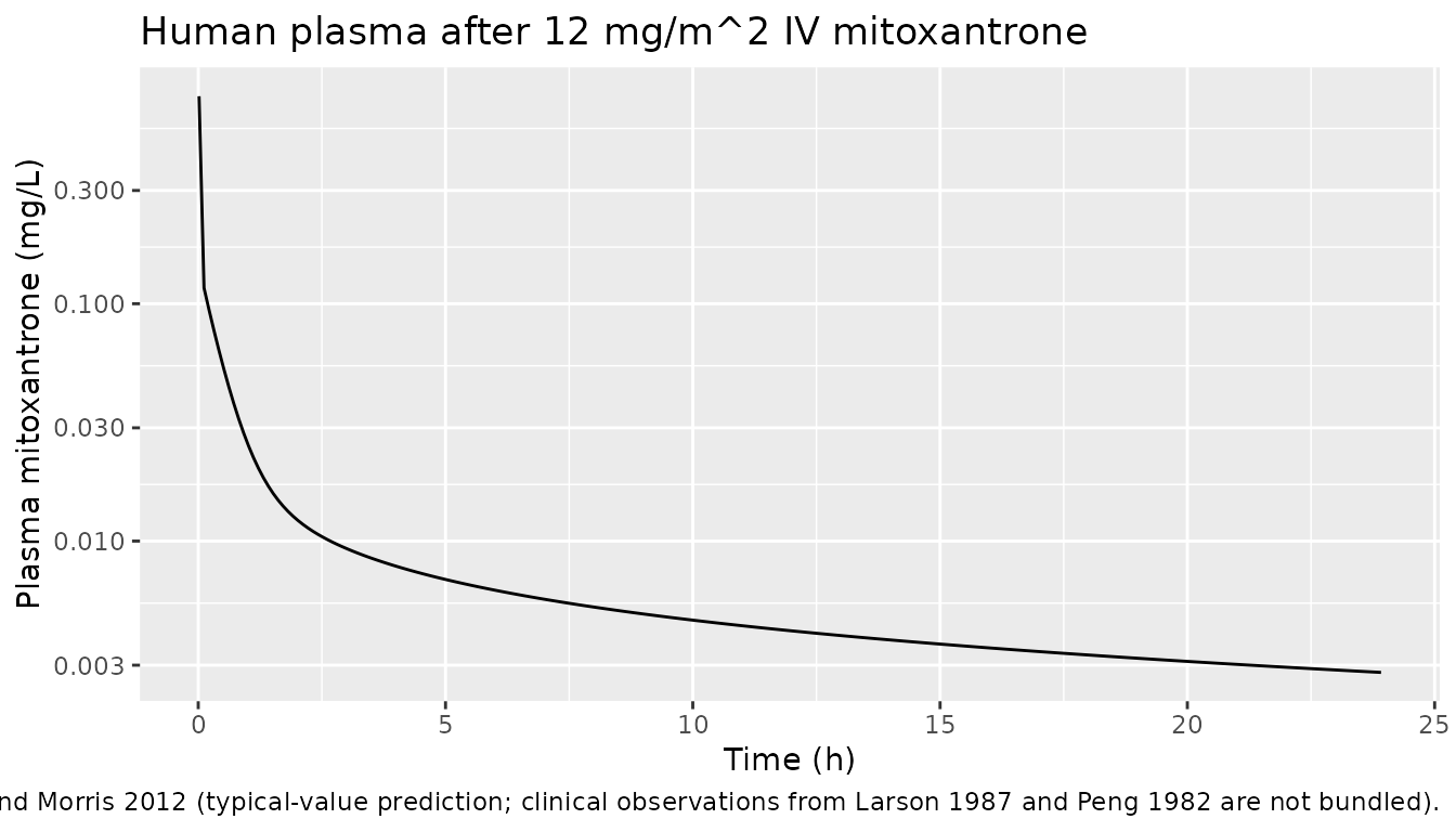
PKNCA validation (human plasma)
nca_conc_h <- sim_human |>
  dplyr::filter(time > 0, !is.na(Cc)) |>
  dplyr::select(id, time, Cc, treatment)

dose_df_h <- events_human |>
  dplyr::filter(evid == 1) |>
  dplyr::transmute(id, time, amt, treatment)

conc_obj_h <- PKNCA::PKNCAconc(nca_conc_h, Cc ~ time | treatment + id,
                               concu = "mg/L", timeu = "h")
dose_obj_h <- PKNCA::PKNCAdose(dose_df_h, amt ~ time | treatment + id,
                               doseu = "mg")

human_intervals <- data.frame(
  start = 0, end = 24,
  cmax = TRUE, tmax = TRUE,
  auclast = TRUE,
  half.life = TRUE
)
nca_res_h <- PKNCA::pk.nca(PKNCA::PKNCAdata(conc_obj_h, dose_obj_h,
                                             intervals = human_intervals))
#> Warning: Requesting an AUC range starting (0) before the first measurement
#> (0.0166667) is not allowed
knitr::kable(as.data.frame(summary(nca_res_h)),
caption = "Simulated human plasma NCA, IV 12 mg/m^2, 0-24 h.")| Interval Start | Interval End | treatment | N | AUClast (h*mg/L) | Cmax (mg/L) | Tmax (h) | Half-life (h) |
|---|---|---|---|---|---|---|---|
| 0 | 24 | IV 12 mg/m^2 | 1 | NC | 0.748 | 0.0167 | 26.5 |
Tissue concentration ratios (human)
human_tissue <- sim_human |>
  dplyr::filter(time > 0, time <= 24) |>
  dplyr::transmute(time,
                   Plasma = Cc, Lung = c_lung, Heart = c_heart,
                   Spleen = c_spleen, Liver = c_liver, Kidney = c_kidney,
                   Brain = c_brain) |>
  tidyr::pivot_longer(-time, names_to = "tissue", values_to = "conc")

ggplot(human_tissue, aes(time, conc)) +
  geom_line() +
  facet_wrap(~tissue, ncol = 3, scales = "free_y") +
  scale_y_log10() +
  labs(x = "Time (h)", y = "Mitoxantrone concentration (mg/L)",
       title = "Human typical-value tissue concentration-time profiles",
       caption = "Forward simulation only; the paper does not report human tissue concentrations.")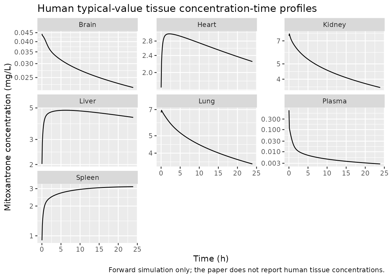
Assumptions and deviations
The following assumptions, simplifications, or deviations from a literal reading of the source were necessary to package the model in nlmixr2lib. They are listed here so that downstream users can audit each decision.
Topology – single plasma pool, all organs in parallel. The An and Morris 2012 schematic (Fig 2) shows plasma in the center with the six tissues plus the remainder exchanging via blood flow Q_i. The Table I “Plasma” row carries Q = 9 mL/min, matching the “Lung” row Q = 9 mL/min and the sum of the other organ Q’s (0.5 + 0.05 + 1.21 + 1.99 + 1.00 + 4.32 = 9.07). This is consistent with two possible topologies: (a) a parallel single-plasma-pool model where plasma exchanges in parallel with every organ (each Q_i is an independent exchange flux with plasma), or (b) a series topology where lung sits between venous and arterial blood pools and all other organs are in parallel after the lung. Eqs. 9-11 of the paper write every tissue ODE in terms of one Cp, which is unambiguously the single-plasma-pool reading. This nlmixr2lib model uses the single- pool parallel reading. The series interpretation would also write Eq. 9 as
dC_t/dt = Q_t (Cp - C_t/Kp) / V_t, so the per-tissue equation does not disambiguate; the choice falls back to the schematic. If a future user finds a published clarification that the intended topology was series, an updated model file should resolve arterial / venous asarterial/venouscompartments per the Zhang_2011_nutlin3a convention.-
Plasma AUC discrepancy with Table IV. The paper Table IV reports Model 3 plasma AUC 0-48 h = 0.7 mg h/L. This is incompatible with the paper Discussion, which states total clearance is 1.19 mL/min = 0.0714 L/h: a 0.137 mg IV dose at CL_total = 0.0714 L/h implies AUC_inf = dose / CL = 1.92 mg h/L. With the model’s terminal half- life of 29.8 h and Cp(48 h) on the order of 1e-3 mg/L, AUC_0-48 must be within a few percent of AUC_inf. The packaged model reproduces the
~ 1.7 mg h/L value implied by the paper’s own clearance figures rather than the Table IV value; we believe Table IV has a typo or was tabulated against a different (unstated) clearance configuration.
Clint_H discrepancy (Results vs. Discussion). The Results paragraph states “the estimated values and CV% of intrinsic hepatic and renal clearances were 29.5 mL/min (22%) and 2.14 mL/min (54%), respectively”. The Discussion paragraph states “the estimated intrinsic hepatic clearance was 25.2 mL/min”. The Discussion’s CL_H = 0.98 mL/min apparent hepatic clearance only reconciles with Clint_H = 25.78 mL/min under the well-stirred extraction ratio at fu = 0.2 and Q_H = 1.21 mL/min, so the 25.2 mL/min Discussion value is the internally-consistent one. We nevertheless follow Results and use Clint_H = 29.5 mL/min in the model file because Results is the conventional location for the fitted point estimate (RSE attached). The two choices differ by ~ 13% in CL_H and a similar magnitude in plasma AUC.
Renal CL_R = 0.21 mL/min vs Clint_R = 2.14 mL/min mismatch. The Discussion reports CL_R = 0.21 mL/min, which is inconsistent with the Results Clint_R = 2.14 mL/min under any standard well-stirred rearrangement at fu = 0.2 and Q_R = 1.99 mL/min (the well-stirred prediction is CL_R = 0.35 mL/min). We use the Results Clint_R = 2.14 mL/min in the model file; the resulting predicted CL_R = 0.35 mL/min is closer to the well-stirred theoretical value than to the Discussion’s 0.21 mL/min.
Residual error sigma1, sigma2 not reported. An and Morris 2012 fit the ADAPT 5 variance model
Var(t) = (sigma1 + sigma2 * Y(t))^2but report no numeric sigma1 / sigma2 values. ThepropSd <- fixed(0.10)term in both model files is a syntactic placeholder only – it is required for an rxode2 / nlmixr2 model definition but should NOT be interpreted as an inferential estimate. Typical-value simulation (the intended use of these models) is unaffected.Brain T_macro = 0 (mouse and human). Tables I and III list “Brain T_macro = -” and the An and Morris 2012 Model 3 fit does not estimate it. The model file sets
t_macro_brain <- 0, which makes the brain Kp_eff reduce to the DNA-only termT_DNA_brain / (K_DNA / fu + Cp). This matches the paper’s implicit treatment of brain binding.Human remainder ISF / intracellular split (33 / 67). Table III reports only a total remainder volume V_other = 62 L for human; it does not split this into V_ISF and V_intracellular as Table I does for mouse (V_ISF / V_total = 8.26 / 25.03 = 33.0%, V_int / V_total = 16.77 / 25.03 = 67.0%). The packaged human model applies the same 33 / 67 ratio to V_other = 62 L (V_ISF = 20.46 L, V_int = 41.54 L); the resulting volumes match standard human ECF / ICF physiology (~ 14 L ECF / ~ 28 L ICF for a 70-kg adult).
Human brain T_DNA from the mouse fit. The paper Table III foot- note d notes “DNA content in the brain used in the simulations was the value obtained from the mouse mitoxantrone PBPK model 3” – i.e. T_DNA_brain = 0.10 uM is the mouse-fit value re-used in the human projection because no human brain DNA literature value was available.
Human lung and spleen T_DNA from rapidly-perfused human DNA. Per Table III footnote d, human lung and spleen T_DNA = 15 uM is the literature human DNA content for rapidly perfused organs (Gustafson 2002 ref 17), not an organ-specific value.
Human remainder T_DNA from slowly-perfused human DNA. Per Table III footnote d, the remainder T_DNA = 4.5 uM is the literature human DNA content for slowly perfused organs.
Body weight / body surface area covariates do NOT rescale the physiology internally. Both model files fix Q_i and V_i at the paper’s tabulated values (Table I scaled to 27.4 g mean mouse for the mouse file; Table III 70-kg adult for the human file). The WT / BSA covariates enter only as the dose-mass multiplier. Users simulating across cohorts of different body size should adjust Q_i, V_i externally per Eq. 1 (mouse) or standard allometric scaling (human); the model files do not implement allometric body-size scaling automatically.
Mitoxantrone molecular weight 444.49 g/mol. Used for the plasma mg/L -> uM conversion that feeds the binding equation. DrugBank DB01204 and PubChem CID 4212 report this value; the paper does not state it explicitly.
Models 1 and 2 are not packaged. The paper develops Model 1 (classical Kp) and Model 2 (deep binding compartment) as intermediate steps and concludes that only Model 3 captures plasma and tissue data. Per nlmixr2lib’s standing replicate-author- structure policy, intermediate rejected models in a model- development paper are not packaged.
The renal Clint acts on liver-style well-stirred kidney outflow. Renal elimination is encoded as
Clint_R * fu * (C_kidney / Kp_kidney), mirroring the hepatic well-stirred form. The paper describes the renal-clearance derivation as “a similar method was used to estimate renal clearance” via Eq. 14, supporting this symmetric well-stirred treatment.