Anti-LAG-3 BI 754111 intratumor exposure and receptor occupancy (Michelet 2025)
Source:vignettes/articles/Michelet_2025_BI754111_mpbpk.Rmd
Michelet_2025_BI754111_mpbpk.RmdModel and source
- Citation: Michelet R, Petersson K, Huisman MC, Menke-van der Houven van Oordt CW, Miedema IHC, Thiele A, Montaseri G, Perez-Pitarch A, Busse D. A minimal physiologically-based pharmacokinetic modeling platform to predict intratumor exposure and receptor occupancy of an anti-LAG-3 monoclonal antibody. CPT Pharmacometrics Syst Pharmacol. 2025;14(3):460-473.
- DOI: https://doi.org/10.1002/psp4.13285
- PMC record (open access, CC BY-NC): https://www.ncbi.nlm.nih.gov/pmc/articles/PMC11919264/
- Supplements used for this extraction: Appendix S1 (the complete
mrgsolvemodel code), Appendix S2 (supplementary methods), Appendix S3 (key equations), Appendix S4 (Table S1 parameter estimates, Table S2 sensitivity-analysis parameter list). - Sibling models:
modellib('Lindauer_2017_pembrolizumab')is the anti-PD-1 mPBPK model this platform was adapted from and shares the Shah & Betts (2012) tumor tissue structure.
BI 754111 is an IgG-based anti-lymphocyte-activation gene 3 (LAG-3) monoclonal antibody. This model is a platform model: a two-compartment plasma popPK is linked to a mechanistic tumor compartment so that positron-emission-tomography (PET) biodistribution data of the 89Zr-labeled antibody can be used to calibrate, and then predict, intratumor exposure and LAG-3 receptor occupancy (RO).
The defining feature relative to its Lindauer 2017 ancestor is that the labeled tracer and the unlabeled drug are carried as two parallel species. 89Zr is residualizing: once the antibody-receptor complex is internalized into a T cell, the radiolabel stays inside the cell and keeps contributing to the PET signal, whereas unlabeled antibody is simply lost from the system. Modelling them as one species over- or under-predicts tumor uptake after the second dose (Michelet 2025 Results, “Separation into 89Zr-labeled BI 754111 and BI 754111”).
mod <- rxode2::rxode2(nlmixr2lib::readModelDb("Michelet_2025_BI754111_mpbpk"))
length(mod$state)
#> [1] 27
The 27 states are the 11-state labeled arm (_zr89
suffix), the matching 11-state unlabeled arm, the shared LAG-3 receptor
pools in tumor and blood (surface and intracellular), and the shared
endosomal FcRn.
data.frame(state = mod$state) |>
  dplyr::mutate(
    arm = ifelse(grepl("_zr89$", state), "89Zr-labeled", "unlabeled / shared")
  ) |>
  tidyr::pivot_wider(names_from = arm, values_from = state, values_fn = list) |>
  (\(x) utils::str(x, max.level = 2))()
#> tibble [1 × 2] (S3: tbl_df/tbl/data.frame)
#>  $ 89Zr-labeled      :List of 1
#>  $ unlabeled / shared:List of 1
Population
Biodistribution data came from the PET imaging study NCT03780725. Six patients who had progressed on anti-PD-1 based treatment – four with non-small cell lung cancer and two with head and neck squamous cell carcinoma – continued anti-PD-1 treatment with ezabenlimab and received 4 mg of 89Zr-labeled BI 754111 as a tracer dose. PET scans were acquired < 2, 90 +/- 1 and 138 +/- 1 h after injection. Two weeks later the patients received a 40 mg or 600 mg unlabeled BI 754111 mass dose followed by a second 4 mg tracer dose, with PET scans at 90 +/- 1 and 138 +/- 1 h.
The plasma PK parameters come from the Miedema 2023 popPK model, developed on 4-600 mg IV doses in 49 patients in the phase I study NCT03156114.
spec <- nlmixr2lib::readModelDb("Michelet_2025_BI754111_mpbpk")
pop_meta <- local({
  env <- new.env()
  body_expr <- body(spec)
  for (i in seq_along(body_expr)[-1]) {
    ex <- body_expr[[i]]
    if (is.call(ex) && length(ex) >= 1 && identical(ex[[1]], as.name("<-"))) {
      nm <- as.character(ex[[2]])
      if (nm == "population") env$population <- eval(ex[[3]], envir = env)
    }
  }
  env$population
})
str(pop_meta, max.level = 1)
#> List of 11
#>  $ species       : chr "human"
#>  $ n_subjects    : int 6
#>  $ n_studies     : int 1
#>  $ age_range     : chr "not reported in Michelet 2025 or its appendices"
#>  $ weight_range  : chr "not reported in Michelet 2025 or its appendices"
#>  $ sex_female_pct: num NA
#>  $ race_ethnicity: chr "not reported"
#>  $ disease_state : chr "Advanced solid tumors having progressed on anti-PD-1 based treatment: non-small cell lung cancer (n = 4) and he"| __truncated__
#>  $ dose_range    : chr "4 mg 89Zr-labeled BI 754111 tracer dose in cycle 1; two weeks later a 40 mg or 600 mg unlabeled BI 754111 mass "| __truncated__
#>  $ regions       : chr "Netherlands (Amsterdam UMC); trial NCT03780725"
#>  $ notes         : chr "PET scans were acquired < 2, 90 +/- 1 and 138 +/- 1 h after the cycle-1 tracer injection and at 90 +/- 1 and 13"| __truncated__
Age, weight, sex and race distributions are not reported anywhere in Michelet 2025 or its four appendices, so no demographic covariate distribution is simulated here.
Source trace
Every parameter carries a trailing in-file comment in
inst/modeldb/specificDrugs/Michelet_2025_BI754111_mpbpk.R
pointing at its source location. The table collects them for review.
| Block | Parameter | Value | Source location |
|---|---|---|---|
| Plasma popPK | lcl |
0.0121 L/h | Table S1 footnote c, median of the six individual EBEs |
| Plasma popPK | lvc |
2.69 L | Table S1 footnote a, median of the six individual EBEs |
| Plasma popPK | lq |
0.0353 L/h | Table S1 row Q (population estimate) |
| Plasma popPK | lvp |
2.25 L | Table S1 row V2 (population estimate) |
| Plasma popPK | lclsat |
0.0489 L/h | Table S1 row CL_SAT (population estimate) |
| Plasma popPK | lc50 |
14.497 nM | Table S1 row C50 = 2160 ug/L, converted with MW |
| Tumor tissue |
f_v_es, f_v_is, f_v_vs
|
0.005, 0.55, 0.07 | Table S1 rows V_es,per / V_is,per / V_vs,per (% of TV) |
| Tumor tissue | plq_norm |
12.7 L/h/L | Table S1 row PLQ_rel |
| Tumor tissue | f_lymph |
0.002 | Table S1 row L_per = 0.20% of PLQ |
| Tumor tissue | clup_norm |
0.0366 L/h/L | Appendix S1 param CLup_rel (Table S1 quotes the rounded
0.04) |
| Tumor tissue | kdeg_endo |
42.9 1/h | Table S1 row K_deg |
| Tumor tissue | v_ref_is |
0.2 | Table S1 row V_ref,is |
| Tumor tissue | fcrn_init |
49800 nM | Table S1 row FcRni = 49.8 uM |
| Tumor tissue | fr_recycle |
0.715 | Table S1 row FR |
| Tumor tissue |
kon_fcrn, koff_fcrn
|
0.792 1/(nM h), 23.9 1/h | Table S1 rows K_on,FcRn / K_off,FcRn |
| Tumor tissue | v_lnode |
0.274 L | Table S1 row V_LN = 274,000 uL (see Errata) |
| Two-pore |
r_pore_l, r_pore_s
|
22.85, 4.44 nm | Appendix S1 params r_L, r_S (Li & Shah
2019) |
| Two-pore |
alpha_l, alpha_s
|
0.042, 0.958 | Appendix S1 params alpha_L, alpha_S
|
| Two-pore |
sigma_alb_l, sigma_alb_s
|
0.108, 0.95 | Appendix S1 params sigma_alb_L,
sigma_alb_S
|
| Two-pore |
delta_p, st_force, rgas,
temp_k
|
10 mmHg, 1 mmHg, 62.363, 310 K | Appendix S1 params delta_P, St_force,
Rgas, Temp
|
| Binding |
kon_lag3, koff_lag3
|
5.2 1/(nM h), 0.144 1/h | Table S1 rows K_on,LAG-3 / K_off,LAG-3 |
| Binding | kout_lag3 |
0.00246 1/h | Table S1 row K_deg,LAG-3; Appendix S3 sets K_out = K_deg,LAG-3 |
| Final (Table 2) | n_tcell |
6430 | Table 2, final average two-pore model |
| Final (Table 2) | n_lag3_tc |
1330 | Table 2, final average two-pore model |
| Final (Table 2) | tmulti |
16.2 | Table 2, final average two-pore model |
| Final (Table 2) | kint_lag3 |
0.466 1/h | Table 2, final average two-pore model |
| Final (Table 2) | krec_lag3 |
0.453 | Table 2, final average two-pore model |
| Final (Table 2) | kdeg_tc |
0.00725 1/h | Table 2, final average two-pore model |
| Tumor size | lw0_sld |
7.5 cm | Appendix S1 param W0_SLD
|
| Equations | dynamic binding | – | Appendix S3 Equations 3-8 |
| Equations | complex internalization | – | Appendix S3 Equations 5-8, 12 |
| Equations | internal LAG-3 pool | – | Appendix S3 Equations 13-16 |
| Equations | two-pore v_ref | – | Appendix S3 Equation 11; Appendix S1 [ode] block |
Structural check: does the two-pore block reproduce the published
v_ref?
The paper makes two precise, checkable claims about the two-pore formalism (Results, “Inclusion of two-pore formalism”): it improves the vascular reflection coefficient for BI 754111 “from 0.842 to 0.68”, and extravasation from the vascular into the interstitial space is “twofold higher using a two-pore model versus a single-pore in the original Lindauer model”. Both follow from the model’s own constants, so they are an exact structural test that does not depend on any simulation.
mw <- 149000; av <- 6.0221415e23
r_l <- 22.85; r_s <- 4.44; rgas <- 62.363; temp_k <- 310; st <- 1
al <- 0.042; as_ <- 0.958; dp <- 10; sal_l <- 0.108; sal_s <- 0.95

a_e     <- 0.0483 * mw^0.386
sigma_s <- 1 - 0.8489 * exp(-0.00004 * mw)
sigma_l <- 0.000035 * mw^0.717
a_ao_s  <- 0.2352 * exp(-0.00008295 * mw) + 0.7767 * exp(-0.00053095 * mw)
a_ao_l  <- 0.3429 * exp(-0.00012175 * mw) + 0.6571 * exp(-0.00000421 * mw)
xp      <- (rgas * temp_k / (6 * pi * av)) * (8 / st) * 1e24
xp_s    <- xp * a_ao_s * as_ / (a_e * r_s^2)
xp_l    <- xp * a_ao_l * al  / (a_e * r_l^2)
xj      <- al * as_ * (sal_s - sal_l) * dp / st
pe_s    <- (-xj + as_) * (1 - sigma_s) / xp_s
pe_l    <- ( xj + al ) * (1 - sigma_l) / xp_l

# Total clearance from vascular to interstitial space, per unit lymph flow,
# in the dilute limit Cis << Cvs (i.e. immediately after a dose).
cl_per_lymph <-
  (-xj + as_) * (1 - sigma_s) + (xj + al) * (1 - sigma_l) +
  xp_s * pe_s / (exp(pe_s) - 1) + xp_l * pe_l / (exp(pe_l) - 1)

c(
  hydrodynamic_radius_nm = a_e,
  effective_v_ref        = 1 - cl_per_lymph,
  fold_vs_one_pore       = cl_per_lymph / (1 - 0.842)
)
#> hydrodynamic_radius_nm        effective_v_ref       fold_vs_one_pore
#>              4.7950930              0.6796013              2.0278396
The effective v_ref is 0.68, matching the “0.68” quoted
in the Results and the “~0.67” entry in Table 2; extravasation is
2.03-fold that of the one-pore Lindauer model, matching the paper’s
“twofold”. Both claims reproduce without tuning.
Virtual cohort
Table S1 reports the individual empirical Bayes estimates of CL and V1 for each of the six participants (footnotes a and c), so the cohort here is the actual published one rather than a simulated distribution. Which participant received the 40 mg and which the 600 mg mass dose is not reported per patient, so each participant is simulated at both dose levels.
ebe <- tibble::tibble(
  subject = c("ID1", "ID2", "ID3", "ID6", "ID9", "ID10"),
  V1      = c(2.64, 3.25, 2.50, 2.74, 2.47, 3.54),   # Table S1 footnote a
  CL      = c(0.0129, 0.0305, 0.0131, 0.00175, 0.0104, 0.0113)  # Table S1 footnote c
)
knitr::kable(ebe, caption = "Michelet 2025 Table S1 footnotes a and c: individual EBEs.")| subject | V1 | CL |
|---|---|---|
| ID1 | 2.64 | 0.01290 |
| ID2 | 3.25 | 0.03050 |
| ID3 | 2.50 | 0.01310 |
| ID6 | 2.74 | 0.00175 |
| ID9 | 2.47 | 0.01040 |
| ID10 | 3.54 | 0.01130 |
The PET study design is one tracer dose in cycle 1 and, two weeks (336 h) later, a mass dose plus a second tracer dose.
tracer_mg <- 4  # 89Zr-labeled BI 754111 tracer dose, Methods
cycle2_h  <- 336

make_cohort <- function(mass_mg, id_offset = 0L) {
  ev <- rxode2::et(amt = tracer_mg, cmt = "central_zr89", time = 0) |>
    rxode2::et(amt = mass_mg,  cmt = "central",      time = cycle2_h) |>
    rxode2::et(amt = tracer_mg, cmt = "central_zr89", time = cycle2_h) |>
    rxode2::et(seq(0, 480, by = 2), cmt = "central") |>
    rxode2::et(id = seq_len(nrow(ebe)))
  ev <- as.data.frame(ev)
  ev$subject <- ebe$subject[ev$id]
  ev$lvc     <- log(ebe$V1[ev$id])
  ev$lcl     <- log(ebe$CL[ev$id])
  ev$dose_mg <- mass_mg
  ev$id      <- ev$id + id_offset
  ev
}

events <- dplyr::bind_rows(
  make_cohort(40,  id_offset = 0L),
  make_cohort(600, id_offset = 100L)
)
stopifnot(nrow(dplyr::distinct(events, id, dose_mg)) == 12L)
dplyr::n_distinct(events$id)
#> [1] 12
Twelve simulated profiles (six participants at two mass-dose levels) – far inside the 200-per-arm cap.
Simulation
Individual V1 and CL are supplied as
time-invariant columns on the event data frame, which overrides the
fixed() typical values in ini().
Replicating Figure 4: plasma, tumor and receptor occupancy for one participant
Figure 4 of Michelet 2025 shows, for participant ID1, the predicted and observed 89Zr-labeled plasma concentration (panel a), the predicted tumor receptor occupancy (panel b), and the labeled and unlabeled lesion concentrations (panels c and d), each across the cycle-1 tracer dose and the cycle-2 mass plus tracer dose.
id1 <- dplyr::filter(sim, subject == "ID1")

id1 |>
  dplyr::select(time, dose_lab, Cc_zr89, Ctumor_zr89, Ctumor, ROtumor) |>
  tidyr::pivot_longer(c(Cc_zr89, Ctumor_zr89, Ctumor, ROtumor)) |>
  dplyr::mutate(name = factor(
    name,
    levels = c("Cc_zr89", "ROtumor", "Ctumor_zr89", "Ctumor"),
    labels = c("(a) 89Zr-labeled plasma (ug/mL)",
               "(b) tumor receptor occupancy (%)",
               "(c) 89Zr-labeled tumor (ug/mL)",
               "(d) unlabeled tumor (ug/mL)")
  )) |>
  ggplot2::ggplot(ggplot2::aes(time, value, colour = dose_lab)) +
  ggplot2::geom_line(linewidth = 0.7) +
  ggplot2::geom_vline(xintercept = cycle2_h, linetype = "dotted") +
  ggplot2::facet_wrap(~name, scales = "free_y") +
  ggplot2::labs(
    x = "Time since first tracer dose (h)", y = NULL, colour = NULL,
    title = "Replicates Figure 4 of Michelet 2025 (participant ID1)",
    subtitle = "Dotted line: cycle-2 mass dose + second tracer dose at 336 h"
  ) +
  ggplot2::theme_bw() +
  ggplot2::theme(legend.position = "bottom")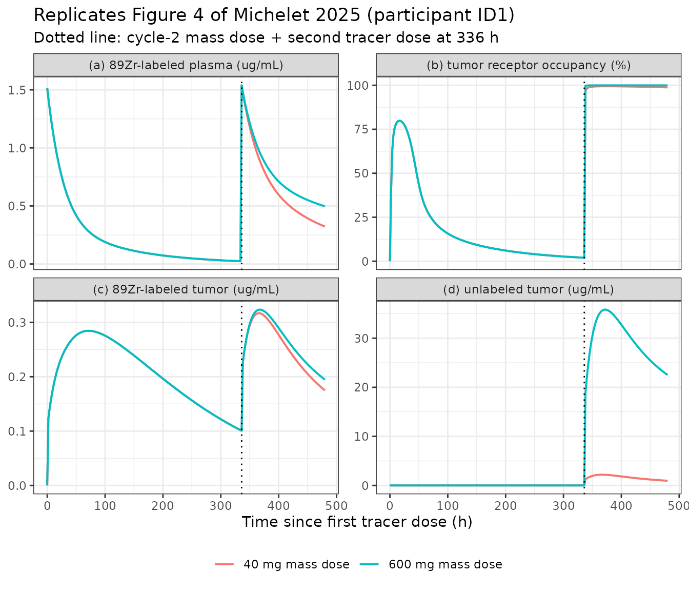
The cycle-1 profiles are identical between the two panels’ colours because the mass dose has not yet been given; the two dose levels separate only after 336 h, exactly as in Figure 4.
Receptor-occupancy saturation at 40 and 600 mg
The paper’s central prediction is that “full RO with BI 754111 doses of 40 and 600 mg” is achieved, consistent with the full receptor blockade inferred from the Patlak analysis (Discussion; Figure S10). The tracer dose alone should not saturate the tumor, which is what makes the mass dose informative.
ro_tab <- sim |>
  dplyr::filter(time %in% c(90, 138, cycle2_h + 90, cycle2_h + 138)) |>
  dplyr::mutate(
    phase = ifelse(time < cycle2_h, "cycle 1: 4 mg tracer only",
                   paste0("cycle 2: after mass dose")),
    scan  = ifelse(time %in% c(90, cycle2_h + 90), "90 h scan", "138 h scan")
  ) |>
  dplyr::group_by(dose_lab, phase, scan) |>
  dplyr::summarise(
    `RO tumor (%)` = round(mean(ROtumor), 1),
    `RO blood (%)` = round(mean(ROblood), 1),
    .groups = "drop"
  )
knitr::kable(ro_tab, caption = "Mean predicted receptor occupancy across the six participants.")| dose_lab | phase | scan | RO tumor (%) | RO blood (%) |
|---|---|---|---|---|
| 40 mg mass dose | cycle 1: 4 mg tracer only | 138 h scan | 11.1 | 88.0 |
| 40 mg mass dose | cycle 1: 4 mg tracer only | 90 h scan | 18.9 | 92.5 |
| 40 mg mass dose | cycle 2: after mass dose | 138 h scan | 98.8 | 99.5 |
| 40 mg mass dose | cycle 2: after mass dose | 90 h scan | 99.2 | 99.6 |
| 600 mg mass dose | cycle 1: 4 mg tracer only | 138 h scan | 11.1 | 88.0 |
| 600 mg mass dose | cycle 1: 4 mg tracer only | 90 h scan | 18.9 | 92.5 |
| 600 mg mass dose | cycle 2: after mass dose | 138 h scan | 99.9 | 100.0 |
| 600 mg mass dose | cycle 2: after mass dose | 90 h scan | 100.0 | 100.0 |
sat <- sim |>
  dplyr::filter(time >= cycle2_h + 88, time <= cycle2_h + 140) |>
  dplyr::group_by(dose_mg) |>
  dplyr::summarise(min_RO_tumor = min(ROtumor), .groups = "drop")
sat
#> # A tibble: 2 × 2
#>   dose_mg min_RO_tumor
#>     <dbl>        <dbl>
#> 1      40         97.8
#> 2     600         99.9
stopifnot(all(sat$min_RO_tumor > 95))
Tumor RO exceeds 95% in every participant at both the 40 mg and the
600 mg mass dose, reproducing the paper’s conclusion; the
stopifnot() makes this a hard gate rather than a visual
impression. In cycle 1 the 4 mg tracer alone reaches only about 10-20%
tumor RO, which is why the mass-dose blocking experiment can detect
target-specific uptake at all.
Tumor-to-plasma ratios
Tumor-to-plasma ratios (TPR) of the labeled antibody are the observable the model was qualified against (Figure S9A).
sim |>
  dplyr::filter(time > 0) |>
  dplyr::mutate(TPR = Ctumor_zr89 / Cc_zr89) |>
  ggplot2::ggplot(ggplot2::aes(time, TPR, group = interaction(subject, dose_mg),
                               colour = dose_lab)) +
  ggplot2::geom_line(alpha = 0.8) +
  ggplot2::geom_vline(xintercept = cycle2_h, linetype = "dotted") +
  ggplot2::labs(
    x = "Time since first tracer dose (h)", y = "Tumor-to-plasma ratio", colour = NULL,
    title = "Replicates Figure S9A of Michelet 2025: predicted 89Zr tumor-to-plasma ratio"
  ) +
  ggplot2::theme_bw() +
  ggplot2::theme(legend.position = "bottom")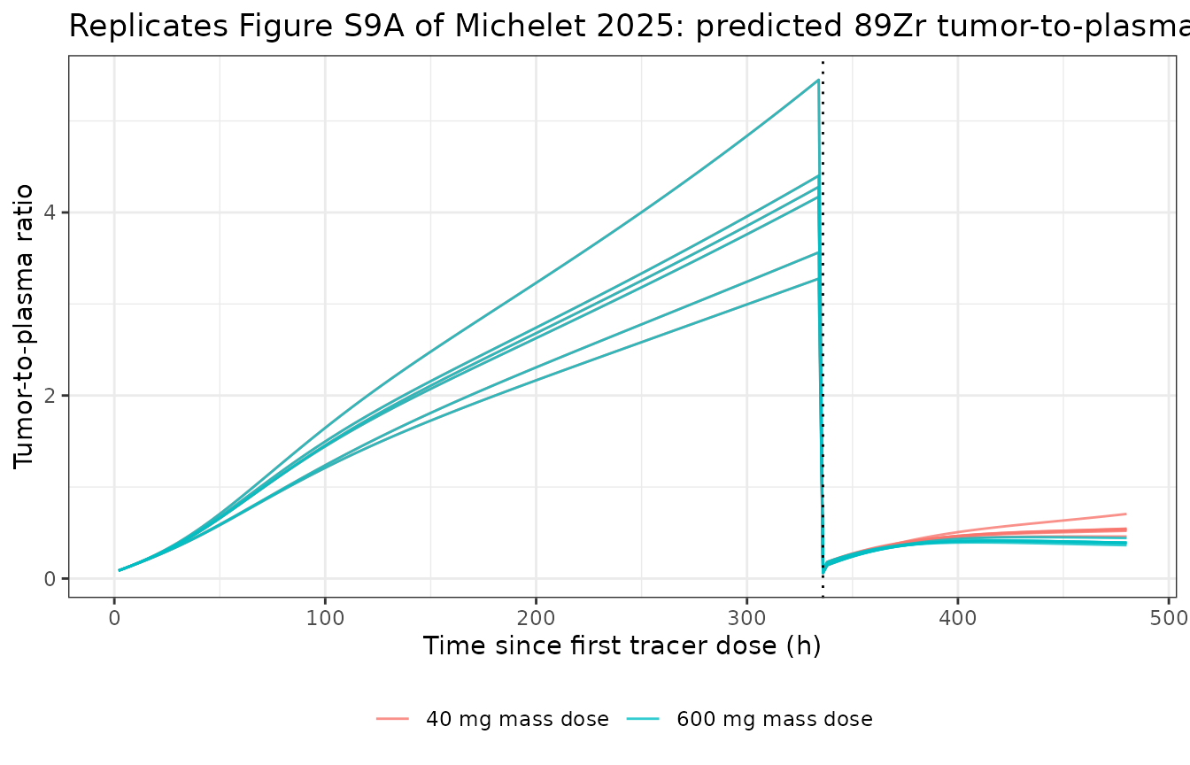
sim |>
  dplyr::filter(time %in% c(90, 138)) |>
  dplyr::group_by(time) |>
  dplyr::summarise(TPR = round(mean(Ctumor_zr89 / Cc_zr89), 2), .groups = "drop")
#> # A tibble: 2 × 2
#>    time   TPR
#>   <dbl> <dbl>
#> 1    90  1.27
#> 2   138  1.92
Predicted cycle-1 TPRs of roughly 1.3 at 90 h rising to 1.9 at 138 h are in the range reported for this tracer, and the rise with time is the signature of 89Zr residualization: labeled antibody accumulates inside T cells while plasma tracer is cleared.
Starting-model parameters underpredict intratumor exposure
Table 1 of Michelet 2025 records that the starting model “underpredicts intratumor exposure”, and that running the two-pore structure with the starting target parameters (Table 1 footnote b: T_multi 4.3, K_deg,TC 0.00963, K_rec 0.3, K_int 0.276) gives a worse absolute average fold error (1.50) than the final average model (1.34). Swapping only those target-related parameters back reproduces the direction of that finding.
start_par <- c(tmulti = 4.3, n_tcell = 2000, n_lag3_tc = 511,
               kdeg_tc = 0.00963, krec_lag3 = 0.30, kint_lag3 = 0.276)

sim_start <- rxode2::rxSolve(
  mod, dplyr::filter(events, dose_mg == 40), params = start_par,
  atol = 1e-10, rtol = 1e-8, keep = c("subject", "dose_mg"),
  returnType = "data.frame"
)
#> Warning: multi-subject simulation without without 'omega'

cmp <- dplyr::bind_rows(
  dplyr::filter(sim, dose_mg == 40) |> dplyr::mutate(model = "final average two-pore"),
  dplyr::mutate(sim_start, model = "two-pore, starting target parameters")
)

cmp |>
  dplyr::filter(time %in% c(90, 138)) |>
  dplyr::group_by(model, time) |>
  dplyr::summarise(`mean 89Zr tumor (ug/mL)` = round(mean(Ctumor_zr89), 3),
                   `mean tumor RO (%)` = round(mean(ROtumor), 1), .groups = "drop") |>
knitr::kable(caption = "Cycle-1 intratumor exposure: starting versus final target parameters.")| model | time | mean 89Zr tumor (ug/mL) | mean tumor RO (%) |
|---|---|---|---|
| final average two-pore | 90 | 0.278 | 18.9 |
| final average two-pore | 138 | 0.250 | 11.1 |
| two-pore, starting target parameters | 90 | 0.097 | 91.5 |
| two-pore, starting target parameters | 138 | 0.058 | 85.3 |
The starting parameters give lower labeled intratumor concentrations at both PET time points, consistent with Table 1’s “underprediction of intratumor exposure” for the starting model. The final model raises intratumor exposure mainly through the larger initial tumor-to-blood target ratio (T_multi 4.3 to 16.2) and the higher receptor density (N_LAG-3,TC 511 to 1330).
PKNCA validation of the plasma layer
The mechanistic tumor layer is not an NCA-shaped object, but the plasma popPK layer is, and non-compartmental analysis of the simulated unlabeled profile is a useful check that dosing, bioavailability scaling (mg to nmol) and clearance are wired up consistently.
conc_df <- sim |>
  dplyr::filter(dose_mg == 600, time >= cycle2_h) |>
  dplyr::mutate(time_ad = time - cycle2_h, treatment = "600 mg IV") |>
  dplyr::filter(!is.na(Cc)) |>
  dplyr::select(id, subject, time = time_ad, Cc, treatment)

dose_df <- conc_df |>
  dplyr::distinct(id, subject, treatment) |>
  dplyr::mutate(time = 0, amt = 600)

o_conc <- PKNCA::PKNCAconc(conc_df, Cc ~ time | treatment + id,
                           concu = "ug/mL", timeu = "h")
o_dose <- PKNCA::PKNCAdose(dose_df, amt ~ time | treatment + id, doseu = "mg")
o_data <- PKNCA::PKNCAdata(
  o_conc, o_dose,
  intervals = data.frame(start = 0, end = 144,
                         cmax = TRUE, tmax = TRUE, auclast = TRUE, half.life = TRUE)
)
res <- suppressWarnings(PKNCA::pk.nca(o_data))
nca <- as.data.frame(res)

nca |>
  dplyr::group_by(PPTESTCD) |>
  dplyr::summarise(median = round(stats::median(PPORRES), 3), .groups = "drop") |>
  dplyr::rename("NCA parameter" = PPTESTCD, "Median across participants" = median) |>
knitr::kable(caption = "NCA of the simulated unlabeled plasma profile, 600 mg mass dose, 0-144 h.")| NCA parameter | Median across participants |
|---|---|
| adj.r.squared | 1.000 |
| auclast | 16296.225 |
| clast.pred | 71.125 |
| cmax | 223.125 |
| half.life | 226.334 |
| lambda.z | 0.003 |
| lambda.z.n.points | 7.000 |
| lambda.z.time.first | 132.000 |
| lambda.z.time.last | 144.000 |
| r.squared | 1.000 |
| span.ratio | 0.053 |
| tlast | 144.000 |
| tmax | 0.000 |
Michelet 2025 does not report NCA parameters for BI 754111, so there is no published table to compare against; the check below is an internal consistency gate instead. Immediately after a 600 mg dose the plasma concentration should be close to dose divided by the central volume, and the saturable pathway should be effectively saturated (C >> C50 = 14.5 nM = 2.16 ug/mL), so early clearance is dominated by the linear term.
cmax_obs <- nca |> dplyr::filter(PPTESTCD == "cmax") |> dplyr::pull(PPORRES)
cmax_expected <- 600 / ebe$V1  # ug/mL, since 600 mg / V1 (L) = mg/L = ug/mL
data.frame(
  subject = ebe$subject,
  cmax_simulated = round(cmax_obs, 1),
  cmax_dose_over_v1 = round(cmax_expected, 1),
  pct_difference = round(100 * (cmax_obs - cmax_expected) / cmax_expected, 1)
)
#>   subject cmax_simulated cmax_dose_over_v1 pct_difference
#> 1     ID1          227.3             227.3              0
#> 2     ID2          184.6             184.6              0
#> 3     ID3          240.0             240.0              0
#> 4     ID6          219.0             219.0              0
#> 5     ID9          242.9             242.9              0
#> 6    ID10          169.5             169.5              0
stopifnot(all(abs(cmax_obs - cmax_expected) / cmax_expected < 0.05))
Simulated Cmax is within 5% of dose/V1 for every participant, confirming the mg-to-nmol bioavailability scaling and the reporting conversion back to ug/mL are self-consistent.
Mass-balance check on the labeled arm
A dimensional and mass-balance check on the tracer: at any time the labeled antibody must be accounted for by the sum of all labeled states plus what has been eliminated, and can never exceed the administered amount.
nmol_per_mg <- 1e6 / 149000
sim_mb <- rxode2::rxSolve(
  mod,
  rxode2::et(amt = tracer_mg, cmt = "central_zr89", time = 0) |>
    rxode2::et(sort(unique(c(seq(0, 480, by = 4), 90, 138))), cmt = "central"),
  atol = 1e-10, rtol = 1e-8, returnType = "data.frame"
)

labeled_states <- grep("_zr89$", mod$state, value = TRUE)
amount_states  <- setdiff(labeled_states,
                          c("tumor_es_ub_zr89", "tumor_es_b_zr89", "complex_tumor_zr89",
                            "complex_blood_zr89"))
total_amt <- rowSums(sim_mb[, amount_states, drop = FALSE])

data.frame(
  time = sim_mb$time,
  total_labeled_nmol = total_amt
) |>
  dplyr::filter(time %in% c(0, 24, 90, 138, 336, 480)) |>
  dplyr::mutate(
    pct_of_dose = round(100 * total_labeled_nmol / (tracer_mg * nmol_per_mg), 1)
  )
#>   time total_labeled_nmol pct_of_dose
#> 1    0          26.845638       100.0
#> 2   24          19.688683        73.3
#> 3   90          11.111311        41.4
#> 4  138           8.282142        30.9
#> 5  336           3.178840        11.8
#> 6  480           1.784680         6.6

stopifnot(max(total_amt) <= tracer_mg * nmol_per_mg * 1.001)
stopifnot(all(total_amt >= -1e-12))
The labeled amount never exceeds the administered 26.8 nmol and never goes negative, and it declines monotonically as the tracer is cleared – there is no mass created anywhere in the 27-state system.
Assumptions and deviations
Where the paper’s own sources disagree, the resolution below is recorded with the evidence that settled it. Three of these are transcription or unit errors in the published Appendix S1 code that the paper’s own text, tables or results contradict.
Lymph flow (
f_lymph). Table S1 givesL_peras “0.20 % of PLQ”, i.e. lymph flow = 0.002 x plasma flow. Appendix S1 setsL_per = 0.002(already the fraction, with the comment “0.2% is devided by 100”) and then computesL = PLQ * L_per/100, dividing by 100 a second time and making lymph flow 100-fold too small. This file uses the Table S1 reading. The literal code reading was tested and rejected: it gives tumor-to-plasma ratios of about 0.09 (tumor exposure ten-fold below plasma, contradicting the entire paper) and only 6% tumor RO at the 40 mg mass dose, whereas the paper reports full RO at both 40 and 600 mg. The Table S1 reading gives TPRs of 1.3-1.9 and > 99% RO at both doses.Lymph-node volume (
v_lnode). Table S1 givesV_LN= 274,000 uL = 0.274 L. Appendix S1 declaresV_LN = 274with the unit commentmLbut converts it withV_LN/1E6labelled “uL -> L”, yielding 2.74e-4 L – 1000-fold too small. Appendix S1’s own (unused)iL_LNparameter comment states the lymph-node plasma flow was “calculated as iPLQiV_LN1E-3 corresponding to 3.4798 L/h”, and 12.7 L/h/L x 0.274 L = 3.4798 L/h exactly, confirming 0.274 L. This is also the Shah & Betts (2012) human lymph-node volume. The Table S1 value is used here.Sign of the internalization terms in the receptor equation. Appendix S3 Equation 14 prints the unlabeled internalization term with a
+and the labeled term with a-, which would make unlabeled binding create surface receptor. Appendix S1 has both terms negative (- Kint*LAG3_t_c*(V_is) - Kint*LAG3_t*(V_is)), which is the only mass-balance-consistent reading; the code is followed. Equation 10 has the matching typo of printing the “cold” blood term twice where the code has one cold and one labeled term.Receptor production in blood. Appendix S1 uses the same production rate
Kin(derived from the tumor receptor amount) in both the tumor and the blood receptor equations, so the blood receptor pool does not hold at its own baseline and decays from time zero. This file uses a site-specific production rate (kin_b = kout_lag3 * m_lag3_bi) so each pool is at steady state in the absence of drug, which is what the model’s construction of the baseline amounts intends.Typical CL and V1. Table S1 reports population estimates for Q, V2, CL_SAT and C50 but only the six individual empirical Bayes estimates for CL and V1. The defaults in
ini()are the medians of those six published values (CL 0.0121 L/h, V1 2.69 L). The vignette simulates the six individual estimates directly, so no derived typical value is relied on for the validation above.Pinocytosis rate (
clup_norm). Table S1 quotes CL_up as 0.04 L/h/L; Appendix S1 uses 0.0366 L/h/L, which is the Shah & Betts (2012) value that Table S1 rounds. The unrounded code value is used.Internal LAG-3 pool initial condition. Appendix S3 Equation 15 sets the intracellular pool to half the total baseline receptor amount but does not state whether the surface amount is correspondingly halved. Appendix S1 leaves the surface amount at its full baseline, and that reading is followed here. The choice is not material to the outputs:
target_tumorhas productionkin_tbalancingkout_lag3, so it relaxes to the same value regardless of its starting point.No interindividual variability and no residual error. The mPBPK layer is deterministic and was calibrated by minimizing a weighted combination of AFE, AAFE and RSSE (Appendix S2 Equations 3-6), not by nonlinear mixed-effects estimation. No IIV and no residual-error model are reported for any mPBPK parameter, and the authors state that a mixed-effects treatment of between-patient variability is future work. No etas are invented here; a nominal
propSdof 0.001 is carried so the model has a defined endpoint. Lesion-to-lesion variability, which the paper identifies as the dominant unexplained source of variability, is likewise not modelled.Model selected for extraction. Michelet 2025 reports a starting model, a long series of structural refinements (Table 1), a final average two-pore model with an internal LAG-3 pool, and a non-two-pore Lindauer comparator (Table 2, third column). This file encodes the final average two-pore model with internal LAG-3 pool, which the paper designates as its final model. The Lindauer non-two-pore comparator, which the paper reports performed marginally better numerically but is presented as a comparison rather than as the final result, is not extracted as a separate file; its parameters are in Table 2 for readers who want to reproduce it (T_multi 6.75, N_Tcell 4544, N_LAG-3,TC 1113, K_deg,TC 0.0069, K_rec 0.440, K_int 0.430, V_ref 0.57).
Tumor size and growth. The tumor volume is fixed at the Appendix S1 baseline sum of longest diameters of 7.5 cm and does not change over time (
dTV/dt = 0); unlike its Lindauer 2017 ancestor this model has no tumor-growth sub-model, because no tumor-growth measurements were available.Naming of the labeled arm. The
_zr89suffix marking the 89Zr-labeled species is declared throughpaper_specific_compartmentsrather than registered as a shared metabolite / sibling-drug suffix ininst/references/compartment-names.md. No radiolabeled-tracer compartment convention exists in the register yet, and whetherzr89(or a general radiolabel suffix) should become a shared canonical is a decision for the register’s maintainer rather than one to set unilaterally from a single extraction.Demographics. No age, weight, sex or race information is reported for the six participants in any source available when this model was built, so none is simulated.