Metoclopramide (Ge 2020) • nlmixr2lib

Model and source

Citation: Ge S, Mendley SR, Gerhart JG, Melloni C, Hornik CP, Sullivan JE, Atz A, Delmore P, Tremoulet A, Harper B, Payne E, Lin S, Erinjeri J, Cohen-Wolkowiez M, Gonzalez D; Best Pharmaceuticals for Children Act - Pediatric Trials Network Steering Committee. Population Pharmacokinetics of Metoclopramide in Infants, Children, and Adolescents. Clin Transl Sci. 2020;13(6):1189-1198. doi:10.1111/cts.12803
Description: Two-compartment population PK model with first-order absorption for metoclopramide in infants, children, and adolescents (Ge 2020), fit simultaneously to opportunistic plasma concentrations after intravenous (bolus or infusion) and enteral (oral, nasogastric, nasojejunal, gastrostomy) dosing. Body weight is the only covariate: clearance and intercompartmental clearance scale allometrically on WT/70 with a fixed exponent of 0.75, and both volumes scale linearly (fixed exponent 1). A single first-order absorption rate and a single bioavailability apply to all enteral routes; interindividual variability is estimated on clearance only, with a proportional residual error.
Article: https://doi.org/10.1111/cts.12803 (open access; PMC7719387)

Ge et al. fit a two-compartment model with first-order absorption to 87 opportunistic plasma metoclopramide concentrations from 50 pediatric patients dosed per standard of care, pooling intravenous and enteral (oral, nasogastric, nasojejunal, gastrostomy) data. Body weight entered a priori with fixed allometric exponents; no other covariate was retained. The final model was then used to simulate steady-state exposure after 0.1 and 0.15 mg/kg orally every 6 hours in virtual patients from term neonates to adolescents (Figures 3 and 4).

Population

The analysis population (Ge 2020 Table 1, Results “Patient characteristics”) was 50 patients enrolled across US Pediatric Trials Network sites in the POPS opportunistic-sampling trial (NCT01431326): 20 infants (postnatal age <= 2 years), 9 children (2-12 years) and 21 adolescents (> 12 years), with median postnatal age 8.89 years (range 0.01-19.13) and median body weight 23.5 kg (5th-95th percentile 2.6-98.1 kg). 52% were male; 70% White, 28% African American and 2% unknown race. Indications (Table S1) were mainly gastroesophageal reflux (18), gastroparesis (9) and headache (8). Twenty patients received an intravenous bolus (median 0.1 mg/kg), 13 received oral doses (median 0.1 mg/kg), and 15 received intravenous, oral and nasogastric/nasojejunal/gastrostomy doses.

The same information is available programmatically via readModelDb("Ge_2020_metoclopramide")()$population.

Source trace

The per-parameter origin is recorded as an in-file comment next to each ini() entry in inst/modeldb/specificDrugs/Ge_2020_metoclopramide.R. The table below collects them in one place.

Equation / parameter	Value	Source location
`lka`	log(0.4) 1/h	Table 2 (Ka); Eq. 5
`lcl`	log(19.6) L/h per 70 kg	Table 2 (CL); Eq. 6
`lvc`	log(42.9) L per 70 kg	Table 2 (Vc); Eq. 7
`lq`	log(57.1) L/h per 70 kg	Table 2 (Q); Eq. 8
`lvp`	log(83.9) L per 70 kg	Table 2 (Vp); Eq. 9
`lfdepot`	log(0.97)	Table 2 (F); Eq. 10
`e_wt_cl_q`	0.75 (fixed)	Methods “Covariate selection”; Results; Eqs. 6 and 8
`e_wt_vc_vp`	1 (fixed)	Methods “Covariate selection”; Results; Eqs. 7 and 9
`etalcl`	0.16501 = log(1 + 0.424^2)	Table 2 (IIV CL 42.4 %CV); Eq. 1
`propSd`	0.333	Table 2 (proportional error 33.3%)
Two-compartment, first-order absorption, no lag	n/a	Results “PopPK model development and evaluation”
One Ka and one F for all enteral routes	n/a	Results (route-specific Ka / F did not improve the fit)
IV doses into `central`, enteral doses into `depot`	n/a	Methods “PopPK analysis” (routes fitted simultaneously)
`Cc = 1000 * central / vc` (ng/mL)	n/a	Methods “Analytical methods” (assay in ng/mL)

Deterministic checks

Steady-state volume

The Discussion reports a typical steady-state volume Vss = Vc + Vp = 1.81 L/kg. With both volumes linear in weight this is weight-independent.

mod <- readModelDb("Ge_2020_metoclopramide")
ini_df <- rxode2::rxode(mod)$iniDf
#> ℹ parameter labels from comments will be replaced by 'label()'
theta <- setNames(ini_df$est, ini_df$name)
vss_per_kg <- (exp(theta[["lvc"]]) + exp(theta[["lvp"]])) / 70
vss_per_kg
#> [1] 1.811429
stopifnot(abs(vss_per_kg - 1.81) < 0.005)

Steady-state AUC over one dosing interval (Eq. 4)

The paper computes AUCss,0-6h as Dose / (CL/F) (Eq. 4). For the typical subject at several body weights, the steady-state profile solved from the ODEs and integrated by PKNCA must equal F * Dose / CL.

mod_typ <- rxode2::zeroRe(mod)
#> ℹ parameter labels from comments will be replaced by 'label()'
wts <- c(3.5, 10, 30, 70)
grid <- seq(0, 6, by = 0.05)
ev_typ <- dplyr::bind_rows(lapply(seq_along(wts), function(i) {
  dplyr::bind_rows(
    data.frame(id = i, time = 0, amt = 0.1 * wts[i], evid = 1L, cmt = "depot",
               ss = 1L, ii = 6),
    data.frame(id = i, time = grid, amt = 0, evid = 0L, cmt = "central",
               ss = 0L, ii = 0)
  ) |>
    dplyr::mutate(WT = wts[i])
}))
sim_typ <- rxode2::rxSolve(mod_typ, events = ev_typ, keep = "WT",
                           rtol = 1e-10, atol = 1e-12,
                           ssRtol = 1e-10, ssAtol = 1e-12, maxsteps = 1e6) |>
  as.data.frame()
#> ℹ omega/sigma items treated as zero: 'etalcl'
#> Warning: multi-subject simulation without without 'omega'

conc_typ <- sim_typ |>
  dplyr::filter(!is.na(Cc)) |>
  dplyr::mutate(Cc = pmax(Cc, 0), treatment = paste0(WT, " kg")) |>
  dplyr::select(id, time, Cc, treatment)
dose_typ <- ev_typ |>
  dplyr::filter(evid == 1) |>
  dplyr::mutate(treatment = paste0(WT, " kg")) |>
  dplyr::select(id, time, amt, treatment)
nca_typ <- PKNCA::pk.nca(PKNCA::PKNCAdata(
  PKNCA::PKNCAconc(conc_typ, Cc ~ time | treatment + id),
  PKNCA::PKNCAdose(dose_typ, amt ~ time | treatment + id),
  intervals = data.frame(start = 0, end = 6, auclast = TRUE, cmax = TRUE)
))

auc_chk <- as.data.frame(nca_typ$result) |>
  dplyr::filter(PPTESTCD == "auclast") |>
  dplyr::select(treatment, auclast = PPORRES) |>
  dplyr::mutate(
    WT = as.numeric(sub(" kg", "", treatment)),
    eq4 = 1000 * exp(theta[["lfdepot"]]) * 0.1 * WT /
      (exp(theta[["lcl"]]) * (WT / 70)^0.75),
    pct_diff = 100 * (auclast / eq4 - 1)
  )
stopifnot(nrow(auc_chk) == length(wts))
auc_chk |>
  dplyr::select(WT, auclast, eq4, pct_diff) |>
  dplyr::rename(
    "Body weight (kg)" = WT,
    "PKNCA AUCss,0-6h (ng*h/mL)" = auclast,
    "Eq. 4 F x Dose / CL (ng*h/mL)" = eq4,
    "Difference (%)" = pct_diff
  ) |>
  knitr::kable(digits = 3,
               caption = "Typical-value AUCss,0-6h after 0.1 mg/kg q6h.")

Typical-value AUCss,0-6h after 0.1 mg/kg q6h.
Body weight (kg)	PKNCA AUCss,0-6h (ng*h/mL)	Eq. 4 F x Dose / CL (ng*h/mL)	Difference (%)
10.0	212.967	212.980	-0.006
3.5	163.802	163.816	-0.008
30.0	280.284	280.298	-0.005
70.0	346.415	346.429	-0.004

# Linear trapezoid on a 0.05 h grid; the residual is integration error only.
stopifnot(max(abs(auc_chk$pct_diff)) < 0.5)

Virtual cohort

Ge 2020 generated 500 virtual patients per postnatal-age group from the PK-Sim European population. PK-Sim is not available here, so weights are drawn from an approximate growth curve: the sex-averaged median weight-for-age of the WHO (0-2 years) and CDC (2-18 years) growth charts, interpolated on age, with log-normal scatter (SD 0.15 on the log scale). Age is drawn uniformly within each group. Following the vignette cohort cap, 200 virtual patients are simulated per age group and regimen.

set.seed(2020)
rxode2::rxSetSeed(2020)

# Sex-averaged median weight-for-age (kg): WHO 0-24 months, CDC 2-18 years.
growth <- data.frame(
  age_y = c(0, 1 / 12, 3 / 12, 6 / 12, 1, 2, 3, 5, 8, 10, 12, 14, 16, 18),
  wt_kg = c(3.3, 4.3, 6.1, 7.6, 9.3, 12.0, 14.2, 18.2, 25.6, 32.3, 40.5, 50.0, 58.5, 63.5)
)

age_groups <- data.frame(
  group = c("< 1 month", "1 month to < 2 years", "2 to < 12 years", "12 to < 18 years"),
  lo = c(0, 1 / 12, 2, 12),
  hi = c(1 / 12, 2, 12, 18)
)
age_groups$group <- factor(age_groups$group, levels = age_groups$group)

n_per_group <- 200L
obs_times <- c(0, 0.25, 0.5, seq(1, 6, by = 0.25))

make_cohort <- function(dose_mgkg, id_offset) {
  subj <- dplyr::bind_rows(lapply(seq_len(nrow(age_groups)), function(g) {
    age <- stats::runif(n_per_group, age_groups$lo[g], age_groups$hi[g])
    data.frame(
      group = age_groups$group[g],
      AGE = age,
      WT = stats::approx(growth$age_y, growth$wt_kg, xout = age)$y *
        exp(stats::rnorm(n_per_group, 0, 0.15))
    )
  }))
  subj$id <- id_offset + seq_len(nrow(subj))
  subj$regimen <- paste0(dose_mgkg, " mg/kg q6h")
  doses <- subj |>
    dplyr::mutate(time = 0, amt = dose_mgkg * WT, evid = 1L, cmt = "depot",
                  ss = 1L, ii = 6)
  obs <- subj |>
    tidyr::crossing(time = obs_times) |>
    dplyr::mutate(amt = 0, evid = 0L, cmt = "central", ss = 0L, ii = 0)
  dplyr::bind_rows(doses, obs) |>
    dplyr::arrange(id, time, dplyr::desc(evid))
}

events <- dplyr::bind_rows(
  make_cohort(0.10, id_offset = 0L),
  make_cohort(0.15, id_offset = 10000L)
)
events$group <- as.character(events$group)
stopifnot(!anyDuplicated(unique(events[, c("id", "time", "evid")])))

Simulation

sim <- rxode2::rxSolve(mod, events = events,
                       keep = c("group", "regimen", "WT"),
                       maxsteps = 1e6) |>
  as.data.frame() |>
  dplyr::mutate(group = factor(group, levels = levels(age_groups$group)))
#> ℹ parameter labels from comments will be replaced by 'label()'
stopifnot(all(sim$Cc >= -1e-6 * max(sim$Cc, na.rm = TRUE), na.rm = TRUE))

The paper reports C_ss,max from simulated concentrations at 0.5, 1, 2, 4 and 6 h after the dose (the sampling times of Kearns 1988), and AUC_ss,0-6h from Eq. 4 (F * Dose / CL, with the individual CL).

f_oral <- exp(theta[["lfdepot"]])
exposure <- sim |>
  dplyr::group_by(id, group, regimen, WT) |>
  dplyr::summarise(
    cssmax = max(Cc[time %in% c(0.5, 1, 2, 4, 6)]),
    cl = cl[1],
    .groups = "drop"
  ) |>
  dplyr::mutate(
    dose = ifelse(regimen == "0.1 mg/kg q6h", 0.1, 0.15) * WT,
    aucss_eq4 = 1000 * f_oral * dose / cl
  )
stopifnot(nrow(exposure) == 2L * nrow(age_groups) * n_per_group)

Replicate published figures

ggplot(exposure, aes(WT, cssmax, colour = group)) +
  geom_point(alpha = 0.5, size = 0.8) +
  geom_hline(yintercept = c(26, 94), linetype = "dashed") +
  geom_hline(yintercept = 143) +
  facet_wrap(~regimen) +
  scale_x_log10() +
  scale_y_log10() +
  labs(x = "Body weight (kg)", y = "Css,max (ng/mL)", colour = "Age group",
       title = "Simulated Css,max vs body weight",
       caption = "Replicates Figure 3 of Ge 2020. Dashed: 26-94 ng/mL; solid: 143 ng/mL.")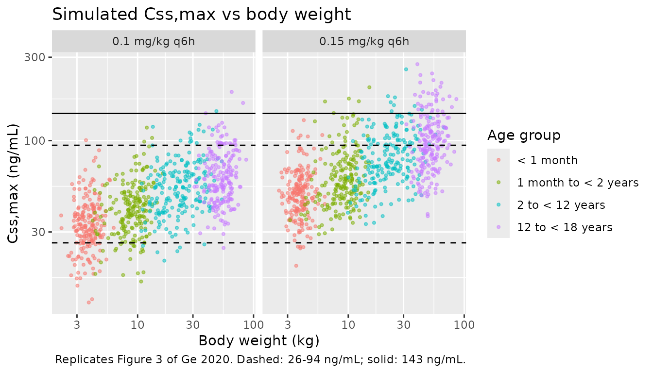

ggplot(exposure, aes(group, aucss_eq4)) +
  geom_boxplot(outlier.size = 0.6) +
  geom_hline(yintercept = c(115, 374), linetype = "dashed") +
  facet_wrap(~regimen) +
  scale_y_log10() +
  labs(x = NULL, y = "AUCss,0-6h (ng*h/mL)",
       title = "Simulated AUCss,0-6h by age group",
       caption = "Replicates Figure 4 of Ge 2020. Dashed: 115-374 ng*h/mL.") +
  theme(axis.text.x = element_text(angle = 20, hjust = 1))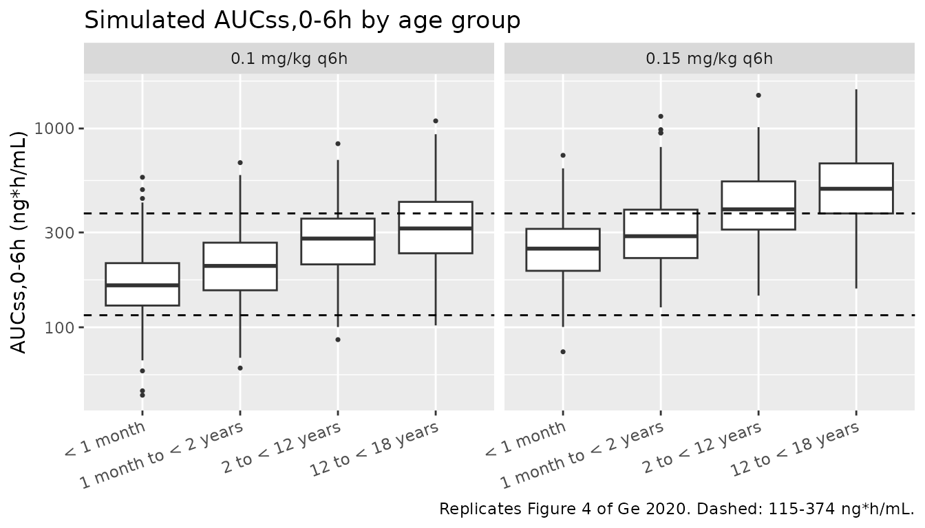

PKNCA validation

PKNCA integrates each simulated steady-state profile (0.25 h grid) over the 0-6 h dosing interval. Its AUC must agree with the paper’s Eq. 4 for every virtual patient, since at steady state the interval AUC equals F * Dose / CL.

sim_nca <- sim |>
  dplyr::filter(!is.na(Cc)) |>
  dplyr::mutate(Cc = pmax(Cc, 0),
                treatment = paste(regimen, group, sep = " | ")) |>
  dplyr::select(id, time, Cc, treatment)
dose_df <- events |>
  dplyr::filter(evid == 1) |>
  dplyr::mutate(treatment = paste(regimen, group, sep = " | ")) |>
  dplyr::select(id, time, amt, treatment)

nca_res <- PKNCA::pk.nca(PKNCA::PKNCAdata(
  PKNCA::PKNCAconc(sim_nca, Cc ~ time | treatment + id),
  PKNCA::PKNCAdose(dose_df, amt ~ time | treatment + id),
  intervals = data.frame(start = 0, end = 6, cmax = TRUE, tmax = TRUE,
                         auclast = TRUE)
))

nca_wide <- as.data.frame(nca_res$result) |>
  dplyr::select(id, treatment, PPTESTCD, PPORRES) |>
  tidyr::pivot_wider(names_from = PPTESTCD, values_from = PPORRES)

chk <- nca_wide |>
  dplyr::inner_join(exposure |> dplyr::select(id, aucss_eq4), by = "id") |>
  dplyr::mutate(pct_diff = 100 * (auclast / aucss_eq4 - 1))
stopifnot(nrow(chk) == nrow(exposure))
# The two sides share each subject's drawn parameters; the difference is
# trapezoid error on the 0.25 h grid (largest for fast-absorbing small infants).
stopifnot(
  abs(median(chk$pct_diff)) < 1,
  max(abs(chk$pct_diff)) < 3
)

nca_wide |>
  dplyr::group_by(treatment) |>
  dplyr::summarise(
    cmax = median(cmax), tmax = median(tmax), auclast = median(auclast),
    .groups = "drop"
  ) |>
  dplyr::rename(
    "Regimen | age group" = treatment,
    "Median Cmax,ss (ng/mL)" = cmax,
    "Median Tmax,ss (h)" = tmax,
    "Median AUCss,0-6h (ng*h/mL)" = auclast
  ) |>
  knitr::kable(digits = 1, caption = "PKNCA steady-state summary by regimen and age group.")

PKNCA steady-state summary by regimen and age group.
Regimen \| age group	Median Cmax,ss (ng/mL)	Median Tmax,ss (h)	Median AUCss,0-6h (ng*h/mL)
0.1 mg/kg q6h \| 1 month to < 2 years	40.3	1.2	203.1
0.1 mg/kg q6h \| 12 to < 18 years	60.6	1.2	313.6
0.1 mg/kg q6h \| 2 to < 12 years	54.0	1.2	279.0
0.1 mg/kg q6h \| < 1 month	32.8	1.2	162.1
0.15 mg/kg q6h \| 1 month to < 2 years	57.6	1.2	286.5
0.15 mg/kg q6h \| 12 to < 18 years	95.4	1.2	496.7
0.15 mg/kg q6h \| 2 to < 12 years	76.5	1.2	391.3
0.15 mg/kg q6h \| < 1 month	50.2	1.2	248.1

Comparison against published results

The paper reports no NCA table; its simulation results are the percentage of virtual patients whose C_ss,max lies within 26-94 ng/mL and whose AUC_ss,0-6h lies within 115-374 ng*h/mL (Results “Dose-response simulation results”).

pct_in <- function(x, lo, hi) 100 * mean(x >= lo & x <= hi)
summ <- function(d) {
  c(cmax = pct_in(d$cssmax, 26, 94), auc = pct_in(d$aucss_eq4, 115, 374))
}
e01 <- dplyr::filter(exposure, regimen == "0.1 mg/kg q6h")
e015 <- dplyr::filter(exposure, regimen == "0.15 mg/kg q6h")
s_all <- summ(e01)
s_inf <- summ(dplyr::filter(e01, group == "1 month to < 2 years"))
s_neo <- summ(dplyr::filter(e015, group == "< 1 month"))
pct_tox_adol <- 100 * mean(
  dplyr::filter(e01, group == "12 to < 18 years")$cssmax > 143
)

comparison <- data.frame(
  quantity = c(
    "0.1 mg/kg, all ages: Css,max in 26-94 ng/mL (%)",
    "0.1 mg/kg, all ages: AUCss,0-6h in 115-374 ng*h/mL (%)",
    "0.1 mg/kg, 1 month to < 2 years: Css,max in range (%)",
    "0.1 mg/kg, 1 month to < 2 years: AUCss,0-6h in range (%)",
    "0.15 mg/kg, < 1 month: Css,max in range (%)",
    "0.15 mg/kg, < 1 month: AUCss,0-6h in range (%)",
    "0.1 mg/kg, 12 to < 18 years: Css,max > 143 ng/mL (%)"
  ),
  published = c(84.3, 75.5, 87.8, 82.6, 94.2, 81.8, 1),
  simulated = c(s_all[["cmax"]], s_all[["auc"]], s_inf[["cmax"]],
                s_inf[["auc"]], s_neo[["cmax"]], s_neo[["auc"]], pct_tox_adol)
)
comparison |>
  dplyr::rename(
    "Quantity" = quantity,
    "Ge 2020" = published,
    "This simulation" = simulated
  ) |>
  knitr::kable(digits = 1, caption = "Percentage of virtual patients within the exposure ranges.")

Percentage of virtual patients within the exposure ranges.
Quantity	Ge 2020	This simulation
0.1 mg/kg, all ages: Css,max in 26-94 ng/mL (%)	84.3	85.6
0.1 mg/kg, all ages: AUCss,0-6h in 115-374 ng*h/mL (%)	75.5	77.0
0.1 mg/kg, 1 month to < 2 years: Css,max in range (%)	87.8	89.0
0.1 mg/kg, 1 month to < 2 years: AUCss,0-6h in range (%)	82.6	85.5
0.15 mg/kg, < 1 month: Css,max in range (%)	94.2	94.5
0.15 mg/kg, < 1 month: AUCss,0-6h in range (%)	81.8	89.0
0.1 mg/kg, 12 to < 18 years: Css,max > 143 ng/mL (%)	1.0	1.5

The percentages depend on the virtual cohort’s weight distribution as well as on the model, and the cohort here is an approximation of the PK-Sim population used by the authors, so the age-group cells (200 virtual patients each) are shown rather than asserted; the two all-ages percentages are asserted to within 10 percentage points. A mis-transcribed clearance, bioavailability or unit would move every exposure by tens of percent; the check below asserts that the median steady-state exposure of the 0.1 mg/kg regimen sits inside both published ranges in every age group, as the paper’s Figures 3a and 4a show.

med_by_group <- e01 |>
  dplyr::group_by(group) |>
  dplyr::summarise(cmax = median(cssmax), auc = median(aucss_eq4),
                   .groups = "drop")
med_by_group
#> # A tibble: 4 × 3
#>   group                 cmax   auc
#>   <fct>                <dbl> <dbl>
#> 1 < 1 month             32.5  163.
#> 2 1 month to < 2 years  40.1  204.
#> 3 2 to < 12 years       53.7  279.
#> 4 12 to < 18 years      60.3  314.
# Realised medians (identical at 2 and 16 solver threads): Css,max 32.5 / 40.1 / 53.7 / 60.3
# ng/mL and AUCss 163 / 204 / 279 / 314 ng*h/mL from youngest to oldest. The
# closest margins (neonatal Css,max vs 26, adolescent AUC vs 374) are about 5-6
# standard errors of a 200-subject median at 42% CV.
stopifnot(
  nrow(med_by_group) == 4L,
  all(med_by_group$cmax > 26 & med_by_group$cmax < 94),
  all(med_by_group$auc > 115 & med_by_group$auc < 374)
)

# The two all-ages percentages pool 800 virtual patients (binomial SE about
# 1.3-1.5 percentage points). Realised 85.6% and 77.0% against the published
# 84.3% and 75.5%; a 10-point band is ~7 SE wide. Mutation check on this
# cohort: clearance x 0.75 drops the AUC percentage to 62.6% (fails here), and
# clearance x 1.33 drops the neonatal median Css,max to 24.4 ng/mL (fails the
# median gate above).
stopifnot(
  abs(s_all[["cmax"]] - 84.3) < 10,
  abs(s_all[["auc"]] - 75.5) < 10
)

Assumptions and deviations

Virtual cohort. The authors drew 500 virtual patients per age group from the PK-Sim (version 7.0) European population. This vignette uses 200 per group with weights from an interpolated sex-averaged WHO/CDC median weight-for-age curve and log-normal scatter (SD 0.15). The percentages in the comparison table therefore differ somewhat from the published ones; the model parameters were not adjusted to reduce the difference.
Age groups. The paper names the groups plotted in Figures 3 and 4 only as “term infants to adolescents” matched to the FDA pediatric age groups. The groups here (< 1 month, 1 month to < 2 years, 2 to < 12 years, 12 to < 18 years) follow the FDA definitions and the ranges quoted in the Results.
Enteral routes. The final model uses one Ka and one F for oral, nasogastric, nasojejunal and gastrostomy dosing (route-specific values did not improve the fit), so all enteral doses go into depot. Intravenous bolus doses go into central; the two continuous infusions in the data set are supported by a rate on a central dose record.
IIV. Only clearance carries interindividual variability. The reported 42.4 %CV was converted to a log-normal variance with omega^2 = log(CV^2 + 1) = 0.16501.
Screened covariates. Serum creatinine was significant after backward elimination but was excluded by the authors (model instability, failed covariance step, and loss of significance after removing one subject), and a < 1 month age-group effect (about 30% lower CL) was dropped in backward elimination. Neither is in the model; both are recorded under covariatesDataExcluded. Table 1 prints serum creatinine in “mg/mL”, which is read as mg/dL.
Errata. No correction notice for this article was found in Europe PMC as of 2026-09-27.