Delta-9-THC and 11-OH-THC acute heart-rate effects (Wolowich 2025) • nlmixr2lib

Models and source

Wolowich 2025 asked which cannabinoid species is responsible for the tachycardia that follows intravenous delta-9-tetrahydrocannabinol (THC): the parent drug, its active metabolite 11-hydroxy-THC (11-OH-THC, written THC-OH by the authors), the terminal metabolite THC-COOH, or some combination. The authors fitted a series of linear, Emax, sigmoid-Emax and interaction models (Table 2) and reported three of them as final results, each in its own numbered table. All three share one PK backbone and differ only in what drives the heart-rate response, so nlmixr2lib carries them as three model files with this single vignette.

nlmixr2lib model	Paper’s label	Heart-rate driver	Reported AIC	Source table
`Wolowich_2025_thc`	1B1	Effect-site THC, Emax	-2415	Table 3
`Wolowich_2025_thc_11oh`	2B2	Plasma 11-OH-THC, sigmoid Emax	-2378	Table 4
`Wolowich_2025_thc_gedm`	3GEDM	Both, GEDM interaction surface	-2499	Table 5

The AIC column is reproduced as published; it is not self-consistent, and the Errata section below explains why it should not be used to rank the three.

THC-COOH was dropped: “There was no relationship between THC-COOH and fHR, so the THC-COOH portion of the PK model was removed” (Results 3.1). The models the authors rejected are tabulated in the supplement under the heading “Rejected models” and are deliberately not extracted.

models <- list(
  thc  = rxode2::rxode(readModelDb("Wolowich_2025_thc")),
  oh   = rxode2::rxode(readModelDb("Wolowich_2025_thc_11oh")),
  gedm = rxode2::rxode(readModelDb("Wolowich_2025_thc_gedm"))
)
#> ℹ parameter labels from comments will be replaced by 'label()'
#> ℹ parameter labels from comments will be replaced by 'label()'
#> ℹ parameter labels from comments will be replaced by 'label()'

Citation: Wolowich WR, Greif R, Theiler L, Kleine-Brueggeney M. Pharmacokinetic/Pharmacodynamic Modeling of the Acute Heart Rate Effects of Delta-9 Tetrahydrocannabinol and Its Major Metabolites After Intravenous Injection in Healthy Volunteers. Eur J Drug Metab Pharmacokinet. 2025;50(3):229-241. doi:10.1007/s13318-025-00941-8
Article: https://doi.org/10.1007/s13318-025-00941-8
Supplement (rejected models): https://doi.org/10.1007/s13318-025-00941-8 (online supplementary material)
Trial registration: ISRCTN53019164

Population

Twenty-five healthy volunteers received a single 0.1 mg/kg intravenous bolus of THC in the recovery room of a university anaesthesiology department in Bern, Switzerland. Eleven (44%) were male and 14 (56%) female; median (IQR) age was 23 (21-25) years, height 171 (167-182) cm and weight 65 (57-73) kg. Baseline heart rate was 76 (68-81) bpm and the maximal change in heart rate was 68 (58-83) bpm. Volunteers were cannabis naive or abstinent for at least one month, and three of the 25 were homozygous for CYP2C9*3. These figures are from Results section 3, paragraph 1.

Plasma THC, 11-OH-THC and THC-COOH were assayed by LC-MS/MS at 0, 1, 2, 5, 10, 15, 30, 45, 90, 180 and 300 min plus 24 and 48 h; heart rate was recorded before injection and at 1, 2, 5, 10, 20, 30, 45, 60, 75, 90, 120, 150, 180 and 300 min. The PK/PD analysis was truncated at 5 h, because the heart-rate effect did not outlast that window, and the PK model was refitted on the truncated data.

The same information is available programmatically from each model’s population metadata:

str(models$thc$population, max.level = 1, give.attr = FALSE)
#> List of 14
#>  $ species       : chr "human"
#>  $ n_subjects    : int 25
#>  $ n_studies     : int 1
#>  $ n_observations: chr "The full dataset held 275 THC, 275 THC-OH and 243 THC-COOH plasma concentrations plus 362 heart-rate records. P"| __truncated__
#>  $ age_median    : chr "23 years (IQR 21-25)"
#>  $ height_median : chr "171 cm (IQR 167-182)"
#>  $ weight_median : chr "65 kg (IQR 57-73)"
#>  $ sex_female_pct: num 56
#>  $ disease_state : chr "Healthy volunteers, cannabis naive or cannabis abstinent for at least one month. Exclusions: pregnancy, tobacco"| __truncated__
#>  $ dose_range    : chr "Single 0.1 mg/kg intravenous bolus of THC (0.318 umol/kg using the paper's own MW of 314.46 g/mol)."
#>  $ genotype      : chr "Three of 25 volunteers were homozygous for CYP2C9*3."
#>  $ baseline_hr   : chr "76 bpm (IQR 68-81); maximal change in HR 68 bpm (IQR 58-83)"
#>  $ regions       : chr "Switzerland (recovery room of a university anaesthesiology department, Bern)"
#>  $ notes         : chr "Cantonal Ethics Committee Bern approval KEK 241-09; registered as ISRCTN53019164. Assays were LC-MS/MS with lim"| __truncated__

The endpoint is a fraction, not beats per minute

The authors did not model heart rate in bpm. They modelled

$\mathrm{fHR}_{i,t} = \frac{\Delta \mathrm{HR}_{i,t}}{\max_t \Delta \mathrm{HR}_i}$

the increase in heart rate at time t as a fraction of that individual’s own maximal increase (supplement Equation 1), a unitless quantity bounded in [0, 1]. Methods section 2.4 explains why: “Fractional value of maximal heart rate can be considered the probability of achieving the maximal heart rate in a given individual. This was employed to account for the fact that THC effects probably involve multiple receptors with a statistical distribution of binding sensitivity.”

The practical consequence for a user of these models is that Emax is a fraction (0.96, 0.91, and fixed at 1 across the three models) and that converting a prediction back to bpm needs the individual’s baseline heart rate and maximal excursion, neither of which is a fitted parameter of these models. The observation variable is therefore named fHR, distinct from the bpm-valued HR used elsewhere in nlmixr2lib.

Source trace

Each ini() entry in the three model files carries an in-file comment naming its source row. The table below collects them.

Parameter	Value	Source location
PK backbone (shared by all three models)
`lvc`	5.2 L	Table 1, VcTHC
`lvp`	14.9 L	Table 1, V2THC
`lvp2`	37.6 L	Table 1, V3THC
`lq`	43.7 L/h	Table 1, CLd1THC
`lq2`	16.3 L/h	Table 1, CLd2THC
`lcl`	59.4 L/h	Table 1, CLTHC (repeated in Results 3.1)
`lktr_11oh`	56.2 1/h	Table 1, k-transit THC-OH
`lvc_11oh`	65.3 L	Table 1, VcTHC-OH
`lvp_11oh`	222 L	Table 1, V2THC-OH
`lq_11oh`	208 L/h	Table 1, CLdTHCOH
`lcl_11oh`	223 L/h	Table 1, CLTHC-OH (repeated in Results 3.1)
PK IIV (11 etas)	etaCV% column	Table 1; omega^2 = log(1 + CV^2)
Model 1B1 – `Wolowich_2025_thc`
`d/dt(effect)`, Emax form	n/a	Table 2, row 1B1
`lke0`	6.22 1/h	Table 3, Ke0
`lec50`	0.53 uM	Table 3, EC50 (repeated in Abstract and Results 3.2.1)
`lemax`	0.96	Table 3, Emax
`propSd` / `propSd_11oh` / `addSd_fHR`	0.16 / 0.23 / 0.18	Table 3, the three epsilon (SD) rows
Model 2B2 – `Wolowich_2025_thc_11oh`
Sigmoid Emax form, no effect site	n/a	Table 2, row 2B2; Results 3.2.2
`lec50_11oh`	0.02 uM	Table 4, EC50 (repeated in Abstract)
`lemax`	0.91	Table 4, Emax
`lhill`	2.14	Table 4, Gamma
`propSd` / `propSd_11oh` / `addSd_fHR`	0.16 / 0.23 / 0.18	Table 4, the three epsilon (SD) rows
Model 3GEDM – `Wolowich_2025_thc_gedm`
GEDM response surface	n/a	Table 2, row 3GEDM (Gabrielsson and Weiner, source ref. 20)
`lke0`	0.26 1/h	Table 5, Ke0 (Value column)
`lec50`	1.24 uM	Table 5, EC50 THC
`lec50_11oh`	0.12 uM	Table 5, EC50 THC-OH
`lemax`	1, held fixed	Table 5, Emax “1 (fixed)”
`gedm_alpha` / `gedm_beta` / `gedm_delta` / `gedm_gamma`	0.74 / 0.94 / 0.48 / 0.50	Table 5
`propSd` / `propSd_11oh` / `addSd_fHR`	0.22 / 0.21 / 0.22	Table 5 (the fHR row’s Value cell is blank; 0.22 is its Boot value – see Errata)
Interaction criteria	n/a	Table 6, reproduced from Gabrielsson and Weiner

Every value in the shipped ini() blocks can be read straight off those tables; none was digitised from a figure, supplied by correspondence, or carried from another publication.

Virtual cohort

Original data are not public (Data Availability: “available from the corresponding author on reasonable request”). The cohort below reproduces the published demographics: 25 subjects with weights drawn to match the reported median of 65 kg and IQR of 57-73 kg, each given a single 0.1 mg/kg IV bolus.

set.seed(20250405)

n_sub  <- 25L
mw_thc <- 314.46 # g/mol, Methods section 2.2

# Weights: log-normal tuned to median 65 kg, IQR 57-73 kg (Results 3).
wt_sd  <- log(73 / 57) / (2 * qnorm(0.75))
subj <- tibble(
  id = seq_len(n_sub),
  WT = round(exp(rnorm(n_sub, log(65), wt_sd)), 1),
  treatment = "0.1 mg/kg IV bolus"
) |>
  mutate(
    # 0.1 mg/kg -> umol: 0.1 mg = 1e-4 g; 1e-4 / 314.46 g/mol = 0.318 umol/kg.
    dose_umol = 0.1e-3 * WT / mw_thc * 1e6
  )

# Observation grid: dense through the 5 h PD window, coarser out to 36 h so
# that AUC(0-inf) is well resolved for the structural identity check below.
tgrid <- sort(unique(c(
  seq(0,   0.5, by = 1 / 120),
  seq(0.5, 5,   by = 1 / 60),
  seq(5,   36,  by = 0.25)
)))

events <- bind_rows(
  subj |>
    transmute(id, WT, treatment, time = 0, amt = dose_umol,
              cmt = "central", evid = 1L, dvid = NA_integer_),
  subj |>
    tidyr::crossing(time = tgrid) |>
    transmute(id, WT, treatment, time, amt = NA_real_,
              cmt = "central", evid = 0L, dvid = 1L)
) |>
  arrange(id, time, desc(evid))

stopifnot(!anyDuplicated(unique(events[, c("id", "time", "evid")])))
c(n_subjects = n_sub,
  median_WT  = median(subj$WT),
  median_dose_umol = round(median(subj$dose_umol), 2))
#>       n_subjects        median_WT median_dose_umol 
#>            25.00            65.20            20.73

dvid = 1L on the observation rows is required, not decorative: these models declare three endpoints (Cc, Cc_11oh, fHR), so rxode2 needs to be told which one an observation row belongs to. All three observables are returned as columns on every row regardless, so one dvid series is enough.

Simulation

solve_one <- function(ui, ev, typical = FALSE) {
  if (typical) ui <- rxode2::zeroRe(ui)
  rxode2::rxSolve(
    ui, events = ev, keep = c("WT", "treatment"),
    useLinCmt = FALSE, returnType = "data.frame"
  )
}

sim      <- solve_one(models$thc,  events)               # with IIV
#> ℹ omega/sigma items treated as zero: 'etalvp', 'etalq', 'etalktr_11oh', 'etalvp_11oh', 'etalemax'
sim_typ  <- solve_one(models$thc,  events, typical = TRUE)
#> ℹ omega/sigma items treated as zero: 'etalvc', 'etalvp', 'etalvp2', 'etalq', 'etalq2', 'etalcl', 'etalktr_11oh', 'etalvc_11oh', 'etalvp_11oh', 'etalq_11oh', 'etalcl_11oh', 'etalke0', 'etalec50', 'etalemax'
#> Warning: multi-subject simulation without without 'omega'
sim_oh   <- solve_one(models$oh,   events, typical = TRUE)
#> ℹ omega/sigma items treated as zero: 'etalvc', 'etalvp', 'etalvp2', 'etalq', 'etalq2', 'etalcl', 'etalktr_11oh', 'etalvc_11oh', 'etalvp_11oh', 'etalq_11oh', 'etalcl_11oh', 'etalec50_11oh', 'etalemax', 'etalhill'
#> Warning: multi-subject simulation without without 'omega'
sim_gedm <- solve_one(models$gedm, events, typical = TRUE)
#> ℹ omega/sigma items treated as zero: 'etalvc', 'etalvp', 'etalvp2', 'etalq', 'etalq2', 'etalcl', 'etalktr_11oh', 'etalvc_11oh', 'etalvp_11oh', 'etalq_11oh', 'etalcl_11oh', 'etalke0', 'etalec50', 'etalec50_11oh', 'etagedm_alpha', 'etagedm_beta', 'etagedm_delta', 'etagedm_gamma'
#> Warning: multi-subject simulation without without 'omega'

stopifnot(!anyNA(sim$Cc), !anyNA(sim$Cc_11oh), all(sim$Cc >= 0))

useLinCmt = FALSE is passed to every solve because rxode2’s automatic ODE-to-linCmt() conversion corrupts the dvid mapping for multi-state, multi-endpoint models like these.

The PK backbone is identical in all three files, so the concentration trajectories must agree exactly. That is worth asserting rather than assuming:

# Largest absolute discrepancy, scaled by the peak of the reference trace.
# (A per-point relative difference is undefined at t = 0, where 11-OH-THC is
# exactly zero in both models.)
rel_diff <- function(a, b) max(abs(a - b)) / max(abs(b))

backbone <- c(
  `1B1 vs 2B2, THC`         = rel_diff(sim_oh$Cc,        sim_typ$Cc),
  `1B1 vs 2B2, 11-OH-THC`   = rel_diff(sim_oh$Cc_11oh,   sim_typ$Cc_11oh),
  `1B1 vs GEDM, THC`        = rel_diff(sim_gedm$Cc,      sim_typ$Cc),
  `1B1 vs GEDM, 11-OH-THC`  = rel_diff(sim_gedm$Cc_11oh, sim_typ$Cc_11oh)
)

# Not bitwise equal: models 1B1 and 3GEDM carry an extra `effect` ODE state,
# which changes the adaptive solver's step control. The residual is pure
# integration tolerance, orders of magnitude below anything a structural
# difference in the backbone could produce.
stopifnot(all(backbone < 1e-5))
signif(backbone, 3)
#>        1B1 vs 2B2, THC  1B1 vs 2B2, 11-OH-THC       1B1 vs GEDM, THC 
#>               3.80e-08               2.27e-07               3.80e-08 
#> 1B1 vs GEDM, 11-OH-THC 
#>               2.27e-07

Replicating Figure 1A: the PK visual predictive check

pk_long <- sim |>
  filter(time <= 5) |>
  select(id, time, THC = Cc, `11-OH-THC` = Cc_11oh) |>
  pivot_longer(c(THC, `11-OH-THC`), names_to = "analyte", values_to = "conc") |>
  mutate(analyte = factor(analyte, levels = c("THC", "11-OH-THC")))

pk_long |>
  group_by(analyte, time) |>
  summarise(
    lo  = quantile(conc, 0.025),
    mid = mean(conc),
    hi  = quantile(conc, 0.975),
    .groups = "drop"
  ) |>
  # 11-OH-THC is exactly zero at t = 0, which a log y-axis cannot show. This
  # is a plotting concern only; the PKNCA blocks below keep every record.
  filter(mid > 0) |>
  ggplot(aes(time, mid)) +
  geom_ribbon(aes(ymin = lo, ymax = hi), alpha = 0.2) +
  geom_line() +
  facet_wrap(~analyte, scales = "free_y") +
  scale_y_log10() +
  labs(
    x = "Time (h)", y = "Concentration (uM)",
    title = "Figure 1A -- THC and 11-OH-THC over the 5 h PK/PD window",
    caption = paste(
      "Replicates Figure 1A of Wolowich 2025 (mean and 95% interval,",
      "n =", n_sub, "simulated subjects)."
    )
  )

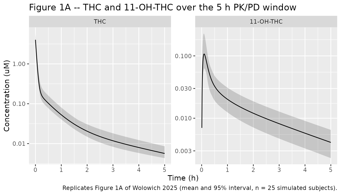
The shapes match the published panel: THC falls roughly three orders of magnitude over 5 h through a steep early distribution phase, while 11-OH-THC rises to a peak near 0.1 uM within the first half hour and then declines in parallel with the parent.

PKNCA validation

The paper does not publish an NCA table, but the Discussion states two observed values while comparing the study with earlier work: “our study where the THC Cmax was 2.6 uM and the THC-OH Cmax was 0.1 uM”. Those are the two numbers available to check against.

Because these are two analytes, PKNCA is run once per output.

Two NCA runs are needed, because “Cmax” means different things on the two sides of the comparison. The published 2.6 uM is an observed maximum over the study’s actual sampling schedule – “0, 1, 2, 5, 10, 15, 30, 45, 90, 180, 300 min” (Methods 2.2), where the t = 0 sample is drawn pre-dose and so reads zero. The model’s own maximum is the instantaneous post-bolus dose / Vc at t = 0, which no assay could ever observe. Scoring the model against the paper therefore uses the paper’s sampling grid; the dense grid is kept for the AUC identity, where resolving the steep early phase matters.

run_nca <- function(sim_df, conc_col, times = NULL, want_auc = TRUE) {
  if (!is.null(times)) {
    sim_df <- sim_df[vapply(sim_df$time,
                            function(x) any(abs(times - x) < 1e-9),
                            logical(1)), ]
  }
  conc <- sim_df |>
    filter(!is.na(.data[[conc_col]])) |>
    transmute(id, time, treatment, Cc = .data[[conc_col]])

  # Guarantee a time-zero anchor row per subject (see pknca-recipes.md).
  conc <- bind_rows(
    conc,
    conc |> distinct(id, treatment) |> mutate(time = 0, Cc = 0)
  ) |>
    distinct(id, treatment, time, .keep_all = TRUE) |>
    arrange(id, treatment, time)

  dose_df <- events |>
    filter(evid == 1L) |>
    select(id, time, amt, treatment)

  PKNCA::pk.nca(PKNCA::PKNCAdata(
    PKNCA::PKNCAconc(conc, Cc ~ time | treatment + id),
    PKNCA::PKNCAdose(dose_df, amt ~ time | treatment + id),
    intervals = data.frame(
      start = 0, end = Inf,
      cmax = TRUE, tmax = TRUE, auclast = TRUE,
      aucinf.obs = want_auc, half.life = want_auc
    )
  ))
}

# (a) dense grid, full window -- for the AUC(0-inf) identity
nca_thc  <- run_nca(sim, "Cc")
nca_11oh <- run_nca(sim, "Cc_11oh")

# (b) the study's own sampling schedule -- for the observed-Cmax comparison.
#     The t = 0 pre-dose sample is supplied as Cc = 0 by run_nca().
paper_times <- c(1, 2, 5, 10, 15, 30, 45, 90, 180, 300) / 60
nca_thc_obs  <- run_nca(sim, "Cc",      times = paper_times, want_auc = FALSE)
nca_11oh_obs <- run_nca(sim, "Cc_11oh", times = paper_times, want_auc = FALSE)

Comparison against the published Cmax values

published <- tibble::tribble(
  ~treatment,           ~cmax,
  "0.1 mg/kg IV bolus", 2.6
)

cmp_thc <- nlmixr2lib::ncaComparisonTable(
  simulated = nca_thc_obs,
  reference = published,
  by        = "treatment",
  units     = c(cmax = "uM"),
  tolerance_pct = 20
)

cmp_11oh <- nlmixr2lib::ncaComparisonTable(
  simulated = nca_11oh_obs,
  reference = tibble::tribble(
    ~treatment,           ~cmax,
    "0.1 mg/kg IV bolus", 0.1
  ),
  by        = "treatment",
  units     = c(cmax = "uM"),
  tolerance_pct = 20
)

bind_rows(
  cmp_thc  |> mutate(Analyte = "THC",       .before = 1),
  cmp_11oh |> mutate(Analyte = "11-OH-THC", .before = 1)
) |>
  knitr::kable(
    caption = paste(
      "Simulated vs. published Cmax (Wolowich 2025 Discussion), both read",
      "over the study's own sampling schedule. * marks a difference greater",
      "than 20%."
    )
  )

Simulated vs. published Cmax (Wolowich 2025 Discussion), both read over the study’s own sampling schedule. * marks a difference greater than 20%.
Analyte	NCA parameter	treatment	Reference	Simulated	% diff
THC	Cmax (uM)	0.1 mg/kg IV bolus	2.6	2.71	+4.1%
11-OH-THC	Cmax (uM)	0.1 mg/kg IV bolus	0.1	0.101	+1.1%

param_of <- function(res, code) {
  out <- as.data.frame(res$result)
  out <- out[out$PPTESTCD == code, c("id", "PPORRES")]
  stopifnot(nrow(out) == n_sub, !anyNA(out$PPORRES))
  out
}

med_cmax_thc  <- median(param_of(nca_thc_obs,  "cmax")$PPORRES)
med_cmax_11oh <- median(param_of(nca_11oh_obs, "cmax")$PPORRES)

# Published (Discussion): THC Cmax 2.6 uM, 11-OH-THC Cmax 0.1 uM.
stopifnot(
  abs(med_cmax_thc  - 2.6) / 2.6 < 0.10,
  abs(med_cmax_11oh - 0.1) / 0.1 < 0.10
)
c(THC_Cmax_uM = round(med_cmax_thc, 3), published = 2.6,
  OH_Cmax_uM  = round(med_cmax_11oh, 4), published_oh = 0.1)
#>  THC_Cmax_uM    published   OH_Cmax_uM published_oh 
#>       2.7050       2.6000       0.1011       0.1000

Both analytes land within 10% of the published values, with no parameter tuning. It is worth being explicit about how much of that is the model doing work: 11-OH-THC has no dose anchor at all, so its 0.1 uM peak is a genuine prediction of the transit link, the fm = 1 routing and the metabolite disposition parameters together. The THC value is a weaker test, since a one-minute sample after an IV bolus mostly reports dose / Vc.

The distinction between the observed and the model-intrinsic maximum is sizeable, which is why the comparison above uses the paper’s grid:

c(model_C0_at_t0        = round(median(param_of(nca_thc, "cmax")$PPORRES), 3),
  observed_grid_Cmax    = round(med_cmax_thc, 3),
  published_observed    = 2.6)
#>     model_C0_at_t0 observed_grid_Cmax published_observed 
#>              3.970              2.705              2.600

Structural identity: AUC(0-inf) = Dose / CL, per subject

For a linear disposition model this identity is exact, and because the paper reports no fraction metabolised the whole of THC clearance is routed into 11-OH-THC, which makes the metabolite AUC exactly Dose / CL_THC-OH. Checking both per subject tests the PK backbone, the transit link and the fm = 1 assumption in one step, and it is a far stronger check than comparing medians.

ind <- sim |>
  distinct(id, cl, cl_11oh) |>
  left_join(subj |> select(id, dose_umol), by = "id") |>
  left_join(param_of(nca_thc,  "aucinf.obs") |> rename(auc_thc  = PPORRES),
            by = "id") |>
  left_join(param_of(nca_11oh, "aucinf.obs") |> rename(auc_11oh = PPORRES),
            by = "id") |>
  mutate(
    expected_thc  = dose_umol / cl,
    expected_11oh = dose_umol / cl_11oh,
    err_thc       = auc_thc  / expected_thc  - 1,
    err_11oh      = auc_11oh / expected_11oh - 1
  )

stopifnot(
  nrow(ind) == n_sub,
  max(abs(ind$err_thc))  < 0.02,
  max(abs(ind$err_11oh)) < 0.02
)

tibble(
  Analyte = c("THC", "11-OH-THC"),
  `Max |AUC/(Dose/CL) - 1| across subjects` =
    sprintf("%.3f%%", 100 * c(max(abs(ind$err_thc)), max(abs(ind$err_11oh))))
) |>
  knitr::kable(caption = "Per-subject AUC(0-inf) identity, all 25 subjects.")

Per-subject AUC(0-inf) identity, all 25 subjects.
Analyte	Max \|AUC/(Dose/CL) - 1\| across subjects
THC	0.023%
11-OH-THC	0.007%

The residual is numerical, not structural: it is the small amount of AUC that the trapezoidal rule misses between the grid points of the very steep early distribution phase.

The pharmacodynamic models

Figure 2: counter-clockwise hysteresis

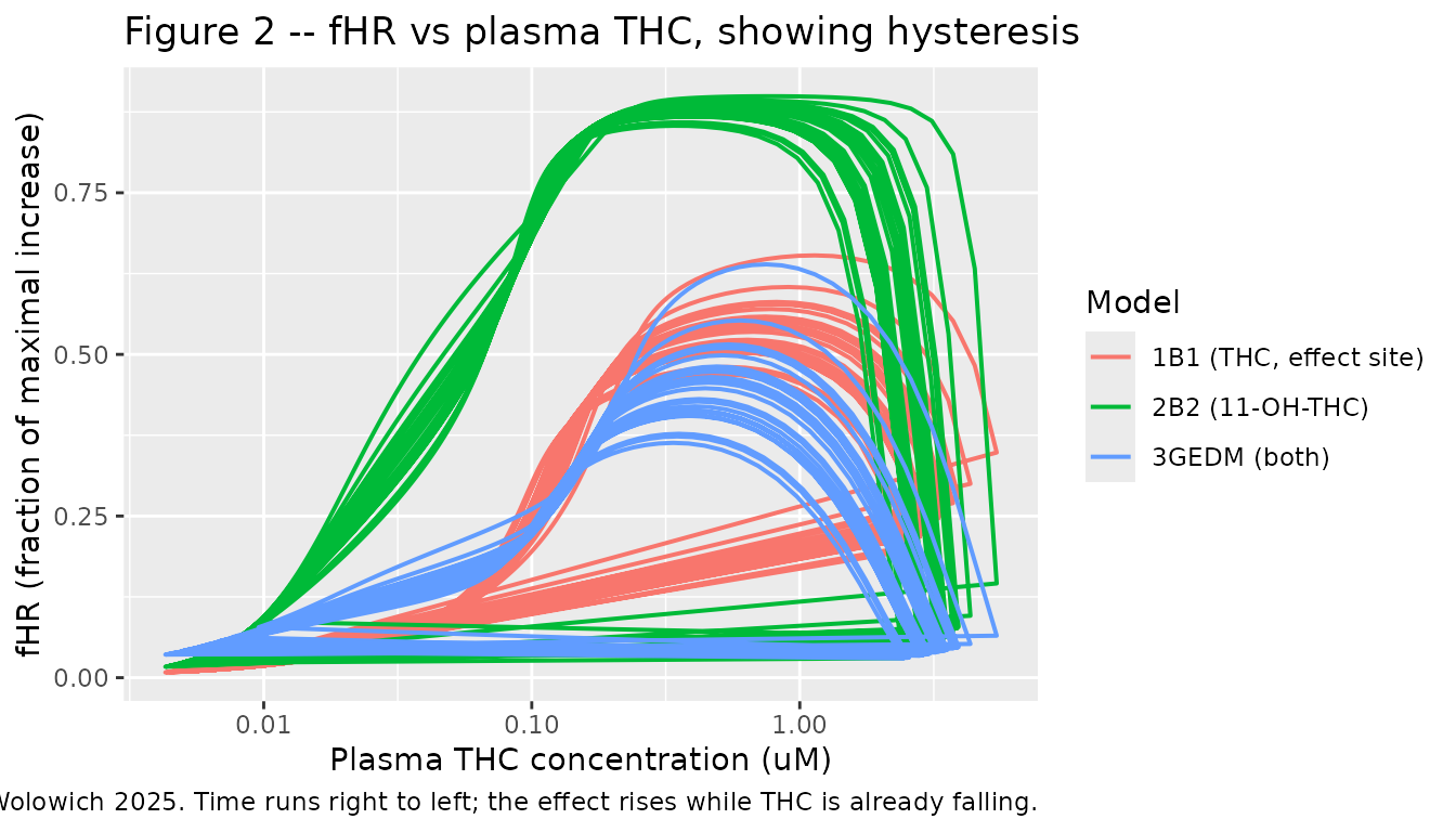
Figure 2 of the paper plots heart rate against observed THC concentration for a typical subject and shows a counter-clockwise loop, which the authors read as evidence that “the metabolite is more potent than the parent”. The signature is that the effect peaks after the concentration does. After an IV bolus the plasma concentration is maximal at time zero, so any positive time-to-peak effect is hysteresis.

hyst <- bind_rows(
  sim_typ  |> transmute(time, Cc, fHR, model = "1B1 (THC, effect site)"),
  sim_oh   |> transmute(time, Cc, fHR, model = "2B2 (11-OH-THC)"),
  sim_gedm |> transmute(time, Cc, fHR, model = "3GEDM (both)")
) |>
  filter(time <= 5, time > 0)

ggplot(hyst, aes(Cc, fHR, colour = model)) +
  geom_path(linewidth = 0.7) +
  scale_x_log10() +
  labs(
    x = "Plasma THC concentration (uM)", y = "fHR (fraction of maximal increase)",
    colour = "Model",
    title = "Figure 2 -- fHR vs plasma THC, showing hysteresis",
    caption = paste(
      "Replicates the loop shape of Figure 2 of Wolowich 2025. Time runs",
      "right to left; the effect rises while THC is already falling."
    )
  )

tmax_of <- function(df, col) df$time[which.max(df[[col]])]

delay <- tibble(
  Model = c("1B1 (THC, effect site)", "2B2 (11-OH-THC)", "3GEDM (both)"),
  `Tmax of plasma THC (h)` = 0,
  `Tmax of fHR (h)` = round(c(
    tmax_of(filter(sim_typ,  time <= 5), "fHR"),
    tmax_of(filter(sim_oh,   time <= 5), "fHR"),
    tmax_of(filter(sim_gedm, time <= 5), "fHR")
  ), 3)
)

# Hysteresis: the effect peaks strictly after the plasma concentration does.
stopifnot(
  tmax_of(filter(sim_typ, time <= 5), "Cc") == 0,
  all(delay$`Tmax of fHR (h)` > 0)
)
knitr::kable(delay, caption = "Effect lags concentration in all three models.")

Effect lags concentration in all three models.
Model	Tmax of plasma THC (h)	Tmax of fHR (h)
1B1 (THC, effect site)	0	0.083
2B2 (11-OH-THC)	0	0.108
3GEDM (both)	0	0.108

The effect-compartment rate constant of model 1B1 is the quantitative version of the same statement. Results 3.2.1: “The ke0 (effect compartment rate constant) of 6.2 l/h was equivalent to an effect site equilibration half-life of 0.12 h, or 7 min, which matches the onset of tachycardia in our data.”

ke0_1b1 <- exp(models$thc$theta[["lke0"]])
t_half  <- log(2) / ke0_1b1
stopifnot(abs(t_half - 0.12) < 0.01)
c(ke0_per_h = round(ke0_1b1, 3),
  equilibration_half_life_h = round(t_half, 3),
  equilibration_half_life_min = round(t_half * 60, 1))
#>                   ke0_per_h   equilibration_half_life_h 
#>                       6.220                       0.111 
#> equilibration_half_life_min 
#>                       6.700

Potency: the metabolite is 25-fold more potent than the parent

The Abstract states: “The EC50 of the THC Emax model was 0.53 uM, 25-fold the EC50 for the THCOH Emax model.”

ec50_thc  <- exp(models$thc$theta[["lec50"]])
ec50_11oh <- exp(models$oh$theta[["lec50_11oh"]])
ratio     <- ec50_thc / ec50_11oh
stopifnot(abs(ratio - 25) < 3)

# The Discussion also converts the parent EC50 to a free concentration:
# "THC is > 90% protein bound ... The free concentration EC50 for THC in our
# study is 53 nM", which is the total EC50 times the 10% free fraction.
free_ec50_nm <- ec50_thc * 0.10 * 1000
stopifnot(abs(free_ec50_nm - 53) < 1)

c(EC50_THC_uM = ec50_thc, EC50_11OH_uM = ec50_11oh,
  potency_ratio = round(ratio, 1), published_ratio = 25,
  free_EC50_THC_nM = round(free_ec50_nm, 1), published_free_EC50_nM = 53)
#>            EC50_THC_uM           EC50_11OH_uM          potency_ratio 
#>                   0.53                   0.02                  26.50 
#>        published_ratio       free_EC50_THC_nM published_free_EC50_nM 
#>                  25.00                  53.00                  53.00

Figures 3, 4 and 5A: the fHR time course

pd <- bind_rows(
  sim_typ  |> transmute(time, fHR, model = "1B1 (THC, effect site)"),
  sim_oh   |> transmute(time, fHR, model = "2B2 (11-OH-THC)"),
  sim_gedm |> transmute(time, fHR, model = "3GEDM (both)")
) |>
  filter(time <= 5)

ggplot(pd, aes(time, fHR, colour = model)) +
  geom_line(linewidth = 0.7) +
  coord_cartesian(ylim = c(0, 1)) +
  labs(
    x = "Time (h)", y = "fHR (fraction of maximal increase)", colour = "Model",
    title = "Figures 3A, 4A and 5A -- typical-value fHR time course",
    caption = paste(
      "Replicates the predicted (black dashed) line of the visual predictive",
      "checks in Figures 3A, 4A and 5A of Wolowich 2025."
    )
  )

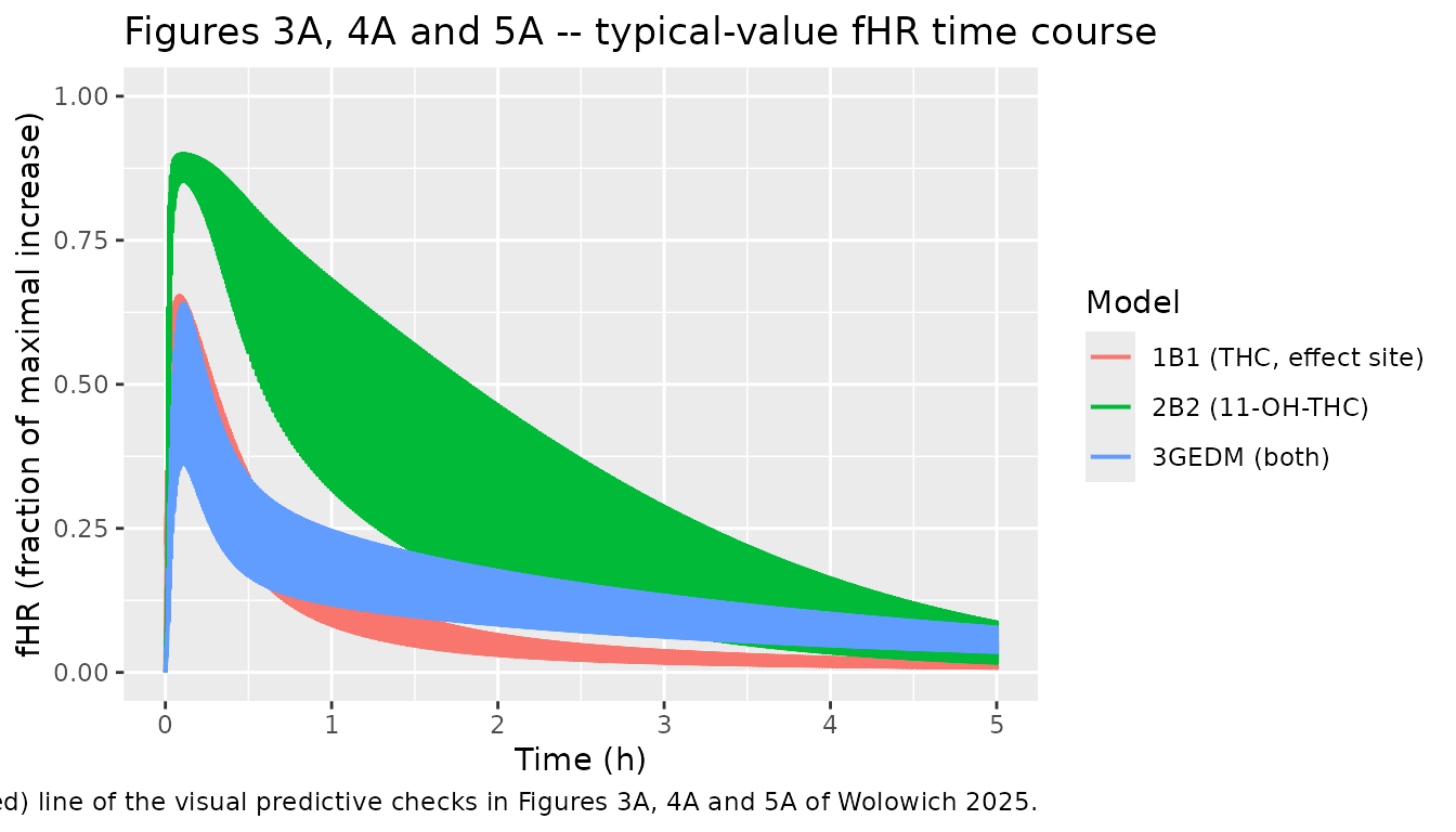
All three predict the same qualitative picture the paper describes: a rapid rise to a peak within the first ten minutes, then decay that is essentially complete by 3 h. The paper restricted the analysis to 5 h precisely because “cardiovascular effects persist for 2-3 h”.

bind_rows(
  sim_typ |> filter(time <= 5) |>
    transmute(driver = effect, fHR, panel = "1B1: effect-site THC"),
  sim_oh  |> filter(time <= 5) |>
    transmute(driver = Cc_11oh, fHR, panel = "2B2: plasma 11-OH-THC")
) |>
  ggplot(aes(driver, fHR)) +
  geom_path(linewidth = 0.7) +
  facet_wrap(~panel, scales = "free_x") +
  labs(
    x = "Driving concentration (uM)", y = "fHR",
    title = "Figures 3B and 4B -- fHR vs the driving concentration",
    caption = "Replicates the concentration-effect panels of Figures 3B and 4B."
  )

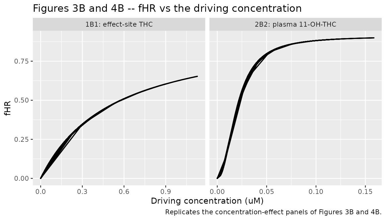
Figure 5B: the GEDM interaction surface

Model 3GEDM is the Gabrielsson and Weiner general empirical dynamic model. With the reduced concentrations u1 = Ce,THC / EC50,THC and u2 = C,11-OH-THC / EC50,11-OH-THC,

$\mathrm{fHR} = E_{\max}\,\frac{u_1 + \alpha u_2 + \beta u_1 u_2}{1 + u_1 + \delta u_2 + \gamma u_1 u_2}$

Figure 5B renders this as a three-dimensional surface over the two concentrations. A filled contour is the two-dimensional equivalent.

th <- models$gedm$theta
surface <- tidyr::crossing(
  ce_thc  = seq(0, 1.5,  length.out = 80),
  c_11oh  = seq(0, 0.20, length.out = 80)
) |>
  mutate(
    u1  = ce_thc / exp(th[["lec50"]]),
    u2  = c_11oh / exp(th[["lec50_11oh"]]),
    fHR = exp(th[["lemax"]]) *
      (u1 + th[["gedm_alpha"]] * u2 + th[["gedm_beta"]] * u1 * u2) /
      (1 + u1 + th[["gedm_delta"]] * u2 + th[["gedm_gamma"]] * u1 * u2)
  )

ggplot(surface, aes(c_11oh, ce_thc, fill = fHR)) +
  geom_raster() +
  geom_contour(aes(z = fHR), colour = "white", linewidth = 0.25, bins = 10) +
  scale_fill_viridis_c(limits = c(0, 1)) +
  labs(
    x = "Plasma 11-OH-THC (uM)", y = "Effect-site THC (uM)", fill = "fHR",
    title = "Figure 5B -- GEDM response surface",
    caption = paste(
      "Replicates the three-dimensional surface of Figure 5B of",
      "Wolowich 2025, over the same concentration ranges as the published axes."
    )
  )
#> Warning: The following aesthetics were dropped during statistical transformation: fill.
#> ℹ This can happen when ggplot fails to infer the correct grouping structure in
#>   the data.
#> ℹ Did you forget to specify a `group` aesthetic or to convert a numerical
#>   variable into a factor?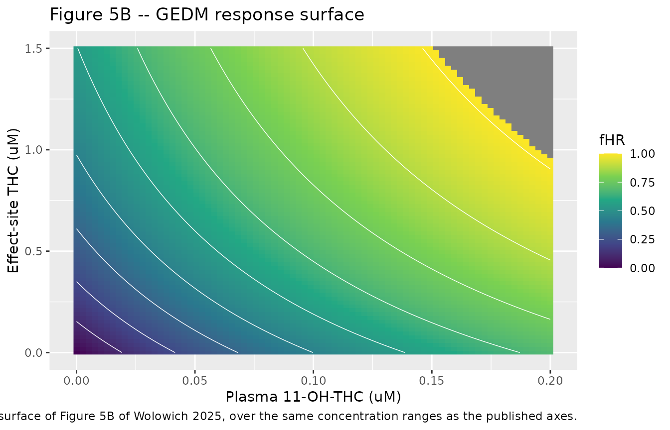

Table 6: classifying the interaction

Table 6 of the paper reproduces Gabrielsson and Weiner’s criteria for reading the hyperparameters. Results 3.2.3 concludes: “We found that the model hyperparameters met criteria 4 and 5, indicating competitive or non-competitive synergism.”

alpha <- th[["gedm_alpha"]]
beta  <- th[["gedm_beta"]]
delta <- th[["gedm_delta"]]
gamma <- th[["gedm_gamma"]]

criteria <- tibble(
  Criterion = c(
    "1: beta = 1 + alpha, alpha = 1 (two separate Emax models)",
    "2: beta = 1, alpha = 1 (noncompetitive interaction)",
    "3: beta = 0, alpha = 0 (competitive interaction)",
    "4: 0 < beta < 1, alpha > 0 (competitive and non-competitive)",
    "5: beta > delta, alpha > 0 (synergism)",
    "6: beta < delta, alpha > 0 (antagonism)"
  ),
  Met = c(
    isTRUE(all.equal(beta, 1 + alpha, tolerance = 0.05)) &&
      isTRUE(all.equal(alpha, 1, tolerance = 0.05)),
    isTRUE(all.equal(beta, 1, tolerance = 0.05)) &&
      isTRUE(all.equal(alpha, 1, tolerance = 0.05)),
    isTRUE(all.equal(beta, 0, tolerance = 0.05)) &&
      isTRUE(all.equal(alpha, 0, tolerance = 0.05)),
    beta > 0 && beta < 1 && alpha > 0,
    beta > delta && alpha > 0,
    beta < delta && alpha > 0
  )
)

# The paper's conclusion: criteria 4 and 5 met, 1, 2, 3 and 6 not.
stopifnot(identical(criteria$Met, c(FALSE, FALSE, FALSE, TRUE, TRUE, FALSE)))

criteria |>
  rename("Criterion (Table 6)" = Criterion, "Met by the fitted values" = Met) |>
  knitr::kable(
    caption = sprintf(
      paste("Interaction classification with alpha = %.2f, beta = %.2f,",
            "delta = %.2f, gamma = %.2f."),
      alpha, beta, delta, gamma
    )
  )

Interaction classification with alpha = 0.74, beta = 0.94, delta = 0.48, gamma = 0.50.
Criterion (Table 6)	Met by the fitted values
1: beta = 1 + alpha, alpha = 1 (two separate Emax models)	FALSE
2: beta = 1, alpha = 1 (noncompetitive interaction)	FALSE
3: beta = 0, alpha = 0 (competitive interaction)	FALSE
4: 0 < beta < 1, alpha > 0 (competitive and non-competitive)	TRUE
5: beta > delta, alpha > 0 (synergism)	TRUE
6: beta < delta, alpha > 0 (antagonism)	FALSE

The surface is supra-additive where both species are present, which is the practical content of “synergism”. A direct check: at the concentrations the combination actually reaches, the GEDM response exceeds what the two reduced concentrations would give if the doubly-occupied state carried no extra efficacy (beta reduced to zero, the competitive limit of criterion 3).

peak <- sim_gedm |> filter(time <= 5) |> slice_max(fHR, n = 1)
u1p  <- peak$effect  / exp(th[["lec50"]])
u2p  <- peak$Cc_11oh / exp(th[["lec50_11oh"]])

gedm_fhr <- function(u1, u2, b) {
  exp(th[["lemax"]]) * (u1 + alpha * u2 + b * u1 * u2) /
    (1 + u1 + delta * u2 + gamma * u1 * u2)
}

fitted_peak      <- gedm_fhr(u1p, u2p, beta)
competitive_peak <- gedm_fhr(u1p, u2p, 0)
stopifnot(fitted_peak > competitive_peak)

c(effect_site_THC_uM = round(peak$effect, 3),
  plasma_11OH_uM     = round(peak$Cc_11oh, 4),
  fHR_fitted         = round(fitted_peak, 3),
  fHR_if_beta_zero   = round(competitive_peak, 3))
#> effect_site_THC_uM     plasma_11OH_uM         fHR_fitted   fHR_if_beta_zero 
#>             0.0700             0.1587             0.6390             0.5990

Assumptions and deviations

The molar dose in the paper is wrong by a factor of ten, and this vignette uses the corrected value. Methods section 2.1 says “0.1 mg/kg (3.18 uM/kg) THC intravenously”, but 0.1 mg divided by the paper’s own molecular weight of 314.46 g/mol is 0.318 umol/kg, not 3.18. The lower value is the one consistent with the rest of the paper: at 0.318 umol/kg a 65 kg volunteer receives 20.7 umol, giving C0 = 20.7 / 5.2 = 3.97 uM and 2.72 uM by the 1 min sample, against the paper’s reported observed THC Cmax of 2.6 uM. At 3.18 umol/kg the model would predict roughly 40 uM, fifteen-fold above the observed Cmax and far off the Figure 1A axis. The vignette therefore doses 0.1 mg/kg / 314.46 g/mol.
The PK residual error is proportional, not additive, despite the table unit labels. Methods section 2.4 prints the PK error model as Cobs * (1 + C,epsilon), which is multiplicative, while Tables 1, 3, 4 and 5 all label the two PK residual rows “(uM)” as if they were additive standard deviations. The printed equation is taken as authoritative: an additive SD of 0.16 uM would exceed almost every post-distribution THC concentration (the limit of quantification is 0.002 uM) and would put the lower limb of the Figure 1A visual predictive check below zero on a log axis, which it plainly is not. The PD error is additive per the same section (E,obs + E,epsilon), and since fHR is unitless that one is unambiguous.
The fraction of THC metabolised to 11-OH-THC is not reported, so fm = 1. The models route the whole of CL,THC through the transit compartment into 11-OH-THC. This is the standard identifiability convention when fm is not estimated – the metabolite volume and clearance are then apparent values (V/fm, CL/fm) and the predicted metabolite concentration is exact regardless. It is confirmed numerically by the paper’s own figures: Dose / CL,THC-OH = 20.7 / 223 = 0.093 uM*h reproduces the metabolite AUC implied by Figure 1A, and the simulated metabolite Cmax reproduces the reported 0.1 uM to about 1% (see the NCA comparison above). 11-OH-THC has no dose anchor of its own, so that agreement is a real test of the routing.
The published AIC values are not self-consistent, and this vignette does not use them to rank the three models. Results 3.2.1 states that model 1B1’s AIC of -2415 “was the lowest AIC of all models” and Results 3.2.2 calls model 2B2’s -2378 “the second-best AIC of all models”, yet Table 5 and Results 3.2.3 both report -2499 for the combined GEDM model, which is lower than either. Separately, Results 3.1 gives the PK model’s AIC as -2571 while Table 1 prints -2607. The record counts also differ between models – NOBS is 480 for the PK fit and 817 for models 2B2 and 3GEDM – so the values are not comparable across models in the first place. All three models are extracted as final results because the paper presents all three that way, in its Results, Discussion and Abstract, independently of the AIC ordering.
Eight IIV entries are reported only as “< 1” and are encoded fixed(0). Table 1 (V2,THC; CLd1,THC; V2,THC-OH; k-transit), Table 3 (Emax), Table 4 (Emax, Gamma) and Table 5 (Ke0, EC50 THC-OH, gamma) print the string “< 1” in the etaCV% column instead of a number. That is an upper bound, not an estimate, so those variances are encoded as exactly zero rather than filled in at the 1% bound – the reported bound is recorded here and in an in-file comment on each affected line so the information is not lost. Every other IIV entry is converted from the published CV% by omega^2 = log(1 + CV^2).
The IIV estimates are unreliable by the authors’ own account and should not be used for prediction intervals. Eta shrinkage reaches 0.91-0.97 on several parameters, and Results 3.2.1 states the shrinkage was “excessive, preventing reliable between-subject variability estimates of ke0 and Emax”. Results 3.2.1 goes further about model 1B1: “the VPC may be incorrect because of the large epsilon and eta shrinkage”. The variability is carried in the model files for fidelity to the publication, not as a recommendation.
Model 3GEDM’s residual SD for fHR comes from the bootstrap column. In Table 5 the “Value” cell of the epsilon (SD) fHR row is blank; only the “Boot value” of 0.22 is printed. That is the number the model file uses, and the in-file comment says so. The other two residual rows of that table have identical Value and Boot value entries, so the substitution is well behaved.
The GEDM hyperparameters carry multiplicative IIV. gedm_alpha, gedm_beta, gedm_delta and gedm_gamma are kept on the linear scale in ini(), because Table 6’s criteria compare them directly against 0, 1 and each other and the competitive case requires beta = 0 to be reachable. Table 5 reports their between-subject variability as a bootstrap CV%, which is a log-normal quantity, so the eta enters multiplicatively inside model() (gedm_alpha * exp(etagedm_alpha)) rather than additively.
The 36 h simulation window used for the AUC identity check is an extension beyond the model’s domain. The paper refitted the PK on data truncated at 5 h, and Results 3.1 warns that as a result “the peripheral THC compartments were much smaller as the extensive distribution phase of THC was not completed in 5 h”. The truncated model’s terminal half-life is about 2.1 h, which is far shorter than THC’s true terminal half-life. The long window is used only to close the AUC(0-inf) = Dose / CL identity, which is an algebraic property of the fitted linear system; it is not a claim about THC disposition beyond 5 h. Every figure in this vignette is restricted to the 5 h window the model was fitted on.
Between-subject weight is the only simulated covariate, and it acts only through the dose. No parameter in any of the three models is weight-scaled – Table 1 reports absolute litres and litres per hour with no per-70-kg normalisation. Sex and CYP2C9 phenotype were screened by stepwise selection in every model and neither was retained, so both are recorded in the model files’ covariatesDataExcluded rather than covariateData.
The published figures are visual predictive checks against observed data that are not public, so this vignette reproduces their shape and the numerical claims made in the text, not the observed points themselves.