Chloroprene PBPK with glutathione depletion (Campbell 2023)
Source:vignettes/articles/Campbell_2023_chloroprene.Rmd
Campbell_2023_chloroprene.RmdModel and source
- Citation: Campbell JL Jr, Clewell HJ III, Van Landingham C, Gentry PR, Andersen ME. (2023). Using available in vitro metabolite identification and time course kinetics for beta-chloroprene and its metabolite, (1-chloroethenyl)oxirane, to include reactive oxidative metabolites and glutathione depletion in a PBPK model for beta-chloroprene. Front Pharmacol 14:1223808. doi:10.3389/fphar.2023.1223808. PMCID PMC10472072. Parent CP distribution/metabolism structure and physiology inherited from Clewell et al. 2019 and Yang et al. 2012 (reproduced in Tables 1, S2, S3, S6). Model code: Supplementary Material, ‘Chloroprene model code for the epoxy submodel’.
- Article: Front Pharmacol 14:1223808
- Supplement (model code, physiological tables, dose-metric summaries): Supplementary Material
Campbell et al. extend the Clewell et al. (2019) physiologically-based pharmacokinetic (PBPK) model for inhaled beta-chloroprene (CP; 2-chloro-1,3-butadiene) to describe the reactive oxidative metabolites formed in lung and liver and the depletion of tissue glutathione (GSH) they cause. Parent CP is distributed over a whole-body flow-limited PBPK structure (lung in series as the portal of entry, then liver, kidney, rapidly- and slowly-perfused tissue and fat) and oxidised by cytochrome P450 to two oxiranes: the stable 1-CEO ((1-chloroethenyl)oxirane) and the unstable 2-CEO. A linked 1-CEO submodel clears 1-CEO by epoxide-hydrolase hydrolysis and, in the mouse only, a second microsomal oxidation to a diepoxide. The unstable 2-CEO and the diepoxide are lumped into a reactive-product (RP) pool that reacts with GSH (second order) and with other cellular constituents (first order). GSH follows zero-order synthesis and first-order turnover, so rising RP production depletes GSH disproportionately as exposure increases.
This article validates the female-mouse
parameterisation (Campbell_2023_chloroprene_mouse_pbpk).
The companion female-rat parameterisation is not shipped: the paper
reports the rat’s 1-CEO, reactive- product and GSH constants (Table 1)
but not the rat parent-CP oxidation Vmax/Km, which reside in the
upstream Clewell et al. (2019) model and are not reproduced here.
Population
The model represents a single reference female B6C3F1 mouse of body weight 0.04 kg (the NTP 1998 time- and survival-weighted average control body weight, Supplementary Table S2). It is a deterministic forward toxicokinetic model, not a fit to individual data, so it carries no between-subject variability and no residual error. Exposures are inhalation of CP vapour at the National Toxicology Program (NTP 1998) bioassay concentrations (0, 12.8, 32 and 80 ppm) over single-6 h and 14-day (6 h/day, 5 days/week) protocols.
The same information is available programmatically via the model’s
population metadata
(readModelDb("Campbell_2023_chloroprene_mouse_pbpk")()$population).
Source trace
Every parameter’s origin is recorded as an in-file comment next to
its ini() entry in
inst/modeldb/specificDrugs/Campbell_2023_chloroprene_mouse_pbpk.R.
The structure (ODEs) was transcribed from the
acslX/Berkeley-Madonna-style listing in the Supplementary Material; the
final values from the tables.
| Group | Parameters | Source |
|---|---|---|
| Physiology (flows, volumes, ventilation, cardiac output) |
qp_per_kg, qcc,
qlc..qrc, vlc..vkc,
vtot_b
|
Supplementary Table S2 (Brown et al. 1997; Marino et al. 2006) |
| Parent-CP partition coefficients |
pb, plu, pl, pf,
ps, pr, pk
|
Supplementary Table S3 (Himmelstein et al. 2004) |
| Parent-CP oxidation kinetics |
vmaxc, km, vmaxclu,
kmlu
|
Supplementary Table S6 (female-mouse central value; Clewell et al. 2019) |
| 1-CEO partition coefficients |
pb1, plu1, pl1,
pf1, ps1, pr1
|
Table 1 (IndusChemFate, logKow 1.22) |
| CP->oxirane split and privileged access |
alphal, alphalu, beta
|
Table 1 (Himmelstein et al. 2004; Campbell et al. 2015) |
| 1-CEO metabolism (hydrolysis + mouse oxidation) |
vmaxc1, km1, vmaxclu1,
kmlu1, vmaxc1o, km1o,
lloxact
|
Table 1 (Himmelstein et al. 2004) |
| Reactive products and GSH |
kgshlc, kgshluc, kfeec,
lleeact, kpc, gso,
gsolu
|
Table 1 (Clewell et al. 2001; D’Souza et al. 1988; Csanady et al. 2003) |
| Rate equations (1-CEO, RP, GSH) | d/dt(...) |
Figure 2, Eqs 1-3; Supplementary model code |
Units note (dimensional analysis). CP and 1-CEO
amounts are in mg; their tissue concentrations
(a_x / (v * p)) are mg/L and feed Michaelis-Menten terms
with Vmax in mg/h and Km in mg/L. The reactive-product and GSH states
are tissue concentrations in uM: RP production converts metabolised mass
to uM/h as (mg/h / (g/mol)) * 1000 / L, the GSH
second-order loss kgsh * RP * GSH has units
(L/umol/h) * (uM) * (uM) = uM/h, and the first-order GSH
turnover kp * GSH has units (1/h) * uM. The
RP->non-GSH term kfee * RP is first order
((1/h) * uM); see the Errata note on its reported unit
label.
Simulation setup
The model is deterministic, so no virtual cohort is required: a
single solve per exposure scenario reproduces the published
typical-value predictions. Inhalation enters through the
conc_air_ppm parameter (a square-wave air concentration);
exp_hours_per_day and exp_days_per_week set
the exposure schedule. Body weight WT is supplied as the
reference female mouse (0.04 kg).
mod <- readModelDb("Campbell_2023_chloroprene_mouse_pbpk")
WT_mouse <- 0.04

# One deterministic solve at a given air concentration and schedule.
solve_cp <- function(ppm, tmax, by = 0.1,
                     hours_per_day = 6, days_per_week = 5) {
  ev <- rxode2::et(seq(0, tmax, by = by))
  rxode2::rxSolve(
    mod,
    c(WT = WT_mouse, conc_air_ppm = ppm,
      exp_hours_per_day = hours_per_day, exp_days_per_week = days_per_week),
    ev, returnType = "data.frame"
  )
}

# Lung and liver GSH baselines (uM) from the model metadata.
GSOLU <- 1500 # lung
GSO <- 7000   # liver
Steady-state and mass-balance checks
With no exposure the model must hold at the reported GSH baselines indefinitely and generate no chloroprene burden.
ss <- solve_cp(ppm = 0, tmax = 336, by = 1)
stopifnot(
  # GSH stays at baseline (deterministic; zero-order synthesis = first-order loss)
  max(abs(ss$Cgsh_lung - GSOLU)) < 1e-4,
  max(abs(ss$Cgsh_liver - GSO)) < 1e-4,
  # no reactive product, no 1-CEO, no systemic CP without exposure
  max(ss$Crp_lung) < 1e-8,
  max(ss$Cc) < 1e-8
)
Chloroprene mass balance over a single 6 h exposure: everything inhaled is accounted for as exhaled + tissue burden + metabolised.
mb <- solve_cp(ppm = 80, tmax = 6, by = 0.05)
e <- mb[nrow(mb), ]
tissue <- with(e, a_lung + a_liver + a_kidney + a_slow + a_rapid + a_fat)
metabolised <- with(e, a_met_liver + a_met_lung)
balance <- e$a_inhaled - (e$a_exhaled + tissue + metabolised)
# relative closure of the chloroprene mass balance
stopifnot(abs(balance) / e$a_inhaled < 1e-3)
Figure 3 – GSH depletion and reactive-product formation vs exposure
Figure 3 shows lung GSH and the reactive-product concentration at the end of a single 6 h exposure as a function of inhaled CP. The paper reports two landmark points for the female mouse: GSH falls 30% below baseline at 6.3 ppm and 50% below baseline at 14.6 ppm (vertical lines in Figure 3).
ppm_grid <- c(seq(0, 20, by = 0.5), seq(22, 120, by = 2))
end6 <- lapply(ppm_grid, function(p) {
  s <- solve_cp(p, tmax = 6, by = 0.1)
  s[nrow(s), c("Cgsh_lung", "Crp_lung")]
})
end6 <- do.call(rbind, end6)
end6$ppm <- ppm_grid
end6$gsh_pct <- 100 * end6$Cgsh_lung / GSOLU
# Landmark depletion points (deterministic; reproduces the Figure 3 verticals).
gsh_at <- function(p) {
  s <- solve_cp(p, tmax = 6, by = 0.1)
  100 * s$Cgsh_lung[nrow(s)] / GSOLU
}
pct_6_3 <- gsh_at(6.3)   # paper: ~70% of baseline (30% depletion)
pct_14_6 <- gsh_at(14.6) # paper: ~50% of baseline (50% depletion)
stopifnot(
  abs(pct_6_3 - 70) < 3,
  abs(pct_14_6 - 50) < 3
)
c(ppm_6.3 = pct_6_3, ppm_14.6 = pct_14_6)
#>  ppm_6.3 ppm_14.6
#> 69.97711 49.86871
ggplot(end6, aes(ppm)) +
  geom_line(aes(y = Cgsh_lung, colour = "Lung GSH (uM)")) +
  geom_line(aes(y = Crp_lung * 500, colour = "Lung RP (uM, x500)")) +
  geom_vline(xintercept = c(6.3, 14.6), linetype = "dashed", colour = "grey50") +
  scale_y_continuous(
    name = "Lung GSH (uM)",
    sec.axis = sec_axis(~ . / 500, name = "Lung reactive product (uM)")
  ) +
  scale_colour_manual(values = c("Lung GSH (uM)" = "#1b7837",
                                 "Lung RP (uM, x500)" = "#2166ac")) +
  labs(x = "Inhaled chloroprene (ppm)", colour = NULL,
       title = "Figure 3 -- end-of-6 h lung GSH and reactive product vs exposure",
       caption = "Replicates Figure 3 of Campbell et al. 2023; dashed lines at 6.3 and 14.6 ppm.") +
  theme(legend.position = "top")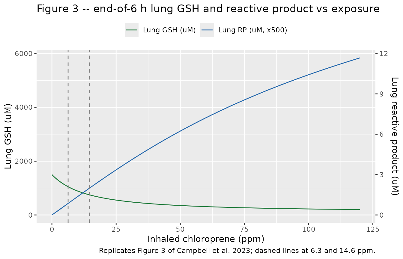
As GSH is consumed the reactive-product concentration rises non-linearly with exposure: once GSH can no longer scavenge the reactive products efficiently they accumulate, the mechanism the paper links to the dose-dependence of toxicity.
Figure 4 – 14-day bioassay timecourse
Figure 4 follows lung CP, 1-CEO, reactive product and GSH over the 14-day bioassay protocol (6 h/day, 5 days/week) at the control and three bioassay concentrations. The square-wave schedule produces rapid rises during each 6 h exposure, partial overnight and weekend recovery of GSH, and progressively deeper GSH depletion over the two weeks at the higher concentrations.
concs <- c(control = 0, `12.8 ppm` = 12.8, `32 ppm` = 32, `80 ppm` = 80)
tc <- lapply(names(concs), function(nm) {
  s <- solve_cp(concs[[nm]], tmax = 336, by = 0.25)
  data.frame(
    time = s$time, exposure = nm,
    CP = s$Cc, `1-CEO` = s$Cceo1_lung,
    RP = s$Crp_lung, GSH = s$Cgsh_lung,
    check.names = FALSE
  )
})
tc <- do.call(rbind, tc)
tc$exposure <- factor(tc$exposure, levels = names(concs))

tc |>
  tidyr::pivot_longer(c("CP", "1-CEO", "RP", "GSH"),
                      names_to = "quantity", values_to = "value") |>
  dplyr::mutate(quantity = factor(quantity, levels = c("CP", "1-CEO", "RP", "GSH"))) |>
  ggplot(aes(time / 24, value, colour = exposure)) +
  geom_line(linewidth = 0.3) +
  facet_wrap(~quantity, scales = "free_y",
             labeller = as_labeller(c(
               CP = "Lung-venous CP (mg/L)", `1-CEO` = "Lung 1-CEO (uM)",
               RP = "Lung reactive product (uM)", GSH = "Lung GSH (uM)"))) +
  labs(x = "Time (days)", y = NULL, colour = "Exposure",
       title = "Figure 4 -- 14-day lung timecourse (6 h/day, 5 days/week)",
       caption = "Replicates Figure 4 of Campbell et al. 2023 (female-mouse lung).")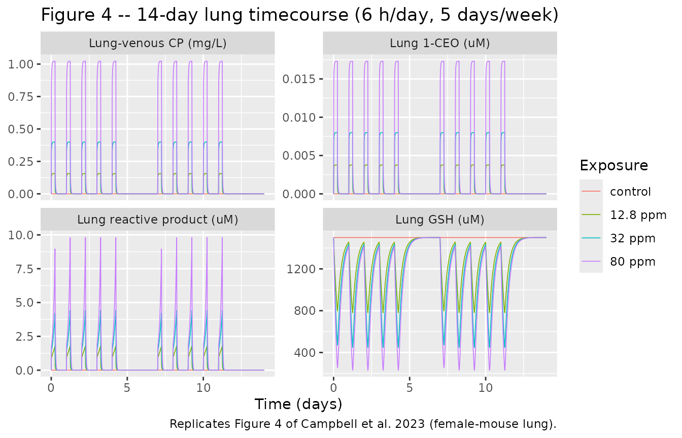
Dose metrics vs Supplementary Table S7
The paper evaluates three candidate lung dose metrics over the 14-day protocol: total CP metabolised per gram lung per day (Tmet), average reactive-product concentration (Preact) and average 1-CEO concentration. Supplementary Table S7 reports Monte-Carlo medians over 1000 parameter draws; the deterministic typical-value model should land near those medians.
MW <- 88.5
TSTOP <- 336
vtot <- 0.0549 + 0.0073 + 0.1 + 0.384 + 0.08098 + 0.0167
vlu <- 0.0073 * WT_mouse * (0.64398 / vtot)

metrics <- lapply(c(12.8, 32, 80), function(p) {
  s <- solve_cp(p, tmax = TSTOP, by = 0.25)
  e <- s[nrow(s), ]
  data.frame(
    ppm = p,
    Tmet = ((e$a_met_lung * 1000 / MW) / (vlu * 1000)) / (TSTOP / 24), # umol/g/day
    Preact = e$auc_rp_lung / TSTOP,       # uM
    CEO1 = e$auc_ceo1_lung / TSTOP        # uM
  )
})
metrics <- do.call(rbind, metrics)

published <- data.frame(
  ppm = c(12.8, 32, 80),
  Tmet_pub = c(0.824, 1.26, 1.61),
  Preact_pub = c(0.247, 0.495, 0.883),
  CEO1_pub = c(5.74e-4, 1.18e-3, 2.51e-3)
)
cmp <- merge(metrics, published, by = "ppm")
cmp |>
  dplyr::transmute(
    "Inhaled (ppm)" = ppm,
    "Tmet (sim)" = round(Tmet, 3), "Tmet (S7 median)" = Tmet_pub,
    "Preact (sim)" = round(Preact, 3), "Preact (S7 median)" = Preact_pub,
    "1-CEO (sim)" = signif(CEO1, 3), "1-CEO (S7 median)" = CEO1_pub
  ) |>
knitr::kable(caption = "Simulated 14-day lung dose metrics vs Supplementary Table S7 medians.")| Inhaled (ppm) | Tmet (sim) | Tmet (S7 median) | Preact (sim) | Preact (S7 median) | 1-CEO (sim) | 1-CEO (S7 median) |
|---|---|---|---|---|---|---|
| 12.8 | 0.855 | 0.824 | 0.250 | 0.247 | 0.000679 | 0.000574 |
| 32.0 | 1.292 | 1.260 | 0.508 | 0.495 | 0.001450 | 0.001180 |
| 80.0 | 1.650 | 1.610 | 0.924 | 0.883 | 0.003130 | 0.002510 |
# Tmet and Preact (the paper's two cross-species-consistent metrics) land
# within ~10% of the Table S7 medians. 1-CEO is more sensitive to the Table 1
# vs Table S6 metabolite-parameter discrepancy and runs ~25% high -- well
# inside its reported ~40% Monte-Carlo CV -- so it carries a wider bound.
stopifnot(
  all(abs(cmp$Tmet - cmp$Tmet_pub) / cmp$Tmet_pub < 0.12),
  all(abs(cmp$Preact - cmp$Preact_pub) / cmp$Preact_pub < 0.12),
  all(abs(cmp$CEO1 - cmp$CEO1_pub) / cmp$CEO1_pub < 0.35)
)
Both Tmet and Preact reproduce the published medians within a few percent, and 1-CEO stays below 0.4% of the reactive-product concentration throughout, matching the paper’s observation that 1-CEO is a minor fraction of total reactive metabolism and a poor cross-species dose metric.
Assumptions and deviations
- Female-rat parameterisation not shipped. The paper gives the rat 1-CEO, reactive-product and GSH constants (Table 1) but not the rat parent-CP oxidation Vmax/Km, which live in the upstream Clewell et al. (2019) model and are not reproduced here. Only the fully-specified female-mouse model is packaged; the rat can be added once the upstream parent-CP kinetics are on hand.
-
Parent-CP oxidation kinetics (
vmaxc,km,vmaxclu,kmlu). These are inherited from Clewell et al. (2019) and taken from the female-mouse central values in Supplementary Table S6, the only source that reports them. -
beta(privileged-access fraction) = 0.33. Table 1 reports 0.33 as the fraction of formed 1-CEO available for distribution/metabolism. The text describes the complementary 67% of butadiene-derived epoxybutene as further metabolised by co-localised epoxide hydrolase (Campbell et al. 2015); the structural term multiplies the available fraction, so 0.33 is used. The supplementary code listing carries 0.67 in the opposite (diverted-fraction) sense; the mouse GSH-depletion curve reproduces Figure 3 only with 0.33 as the available fraction. -
kfeecunit. The maintainers read Table 1’s unit label for KFEEC (L/umol/h) as a copy of the neighbouring KGSH unit: the text states KFEE is a first-order rate constant, Figure 2 Eq 2 uses it first order, and the rate equation is dimensionally consistent only if KFEE is 1/h. The value 35 is therefore applied as a first-order rate (1/h). - Table 1 vs Table S6 metabolite parameters. The 1-CEO hydrolysis and oxidation Vmax/Km differ by about 15-18% between Table 1 (used here, as the explicit “parameters used in the CP metabolite submodel”) and the Table S6 Monte-Carlo central values. This is the main source of the ~25% high 1-CEO dose metric; Tmet and Preact are unaffected.
- Deterministic, no variability. The model is a recoded literature PBPK model evaluated against in vitro kinetics and bioassay dose-response, not a fit to individual data, so it carries no IIV and no residual error. The Supplementary Table S6/S7 Monte-Carlo analysis varies the parameters for an uncertainty assessment but is not between-subject variability.
-
Convention deviations. As a whole-body PBPK model
it uses descriptive per-tissue state names (declared via
paper_specific_compartment_pattern) and non-log-transformed physiological constants rather than the canonical PK parameterisation; both are standard for the PBPK models in this library. - No correction notice for this article was found as of 2026-10-27.