Rivaroxaban (Singkham 2022)
Source:vignettes/articles/Singkham_2022_rivaroxaban.Rmd
Singkham_2022_rivaroxaban.RmdModel and source
- Citation: Singkham N, Phrommintikul A, Pacharasupa P, Norasetthada L, Gunaparn S, Prasertwitayakij N, Wongcharoen W, Punyawudho B. Population Pharmacokinetics and Dose Optimization Based on Renal Function of Rivaroxaban in Thai Patients with Non-Valvular Atrial Fibrillation. Pharmaceutics. 2022;14(8):1744. doi:10.3390/pharmaceutics14081744. PMCID: PMC9414338.
- Description: One-compartment population PK model with first-order absorption and first-order elimination for oral rivaroxaban in Thai adults with non-valvular atrial fibrillation (Singkham 2022). Apparent clearance carries a power effect of Cockcroft-Gault creatinine clearance normalised to 57.5 mL/min and apparent volume a power effect of body weight normalised to 63 kg. Between-subject variability on CL/F and ka only (none on V/F); additive residual error. Concentrations are rivaroxaban-calibrated anti-factor-Xa activity.
- Article: https://doi.org/10.3390/pharmaceutics14081744 (open access, PMC9414338)
Population
Singkham 2022 analysed 240 rivaroxaban-calibrated anti-factor-Xa
concentrations from 60 Thai adults with non-valvular atrial fibrillation
treated at a tertiary hospital in Chiang Mai between June 2018 and
January 2019 (Methods section 2.1; Table 1). Mean (SD) age was 69.4
(9.2) years, body weight 64.0 (14.1) kg and Cockcroft-Gault creatinine
clearance 59.0 (22.8) mL/min; 63.3% were male. Patients with CrCl <
15 mL/min were excluded. Every patient took the standard once-daily dose
(20 mg for CrCl >= 50 mL/min, 15 mg for CrCl 15-49 mL/min) for at
least a week and then the lower Japan-specific dose (15 mg and 10 mg
respectively) for at least a week. Steady-state peak (2-4 h) and trough
(22-24 h) samples were drawn on each regimen, so the data carry little
information on absorption; ka and its variability were therefore
stabilised with a frequentist $PRIOR taken from an earlier
Japanese population PK study.
The same information is available programmatically via
readModelDb("Singkham_2022_rivaroxaban")()$population.
Source trace
| Equation / parameter | Value | Source location |
|---|---|---|
| Structure: one compartment, first-order absorption and elimination | n/a | Results section 3.1 |
lka |
log(0.697) 1/h | Table 2, ka |
lcl |
log(4.19) L/h | Table 2, CL/F |
lvc |
log(37.5) L | Table 2, V/F |
e_crcl_cl |
0.277 | Table 2, CrCl on CL/F; footnote c (Results text prints 0.278) |
e_wt_vc |
0.412 | Table 2, WT on V/F; footnote d |
cl = exp(lcl + etalcl) * (CRCL / 57.5)^e_crcl_cl |
n/a | Table 2 footnote c |
vc = exp(lvc) * (WT / 63)^e_wt_vc |
n/a | Table 2 footnote d; no IIV on V/F (Discussion) |
etalcl |
0.0470 (21.94% CV) | Table 2, IIV of CL/F; omega^2 = log(1 + CV^2) |
etalka |
0.455 (75.91% CV) | Table 2, IIV of ka; omega^2 = log(1 + CV^2) |
addSd |
0.092 mg/L | Table 2, RUV additive; Methods section 2.3 |
Typical-value check against Figure 5
Figure 5 plots the simulated steady-state AUC0-24 by CrCl band. AUC0-24 at steady state equals dose / (CL/F) and does not depend on weight, so the typical-patient value at each band’s midpoint can be compared with the medians read off the Figure 5 boxplots. The maintainers digitised the medians to about +/- 50 ng*h/mL.
mod <- readModelDb("Singkham_2022_rivaroxaban")
ui <- rxode2::rxode(mod)
#> ℹ parameter labels from comments will be replaced by 'label()'
th <- setNames(ui$iniDf$est, ui$iniDf$name)

bands <- tibble(
  crcl_band = factor(c("15-29", "30-49", "50-69", "70-89", "90-110"),
                     levels = c("15-29", "30-49", "50-69", "70-89", "90-110")),
  crcl_mid = c(22, 39.5, 59.5, 79.5, 100)
)
# Medians read off Figure 5 panels A-C (ng*h/mL).
fig5 <- tibble::tribble(
  ~crcl_band, ~dose, ~fig5_median,
  "15-29",  10, 3150, "30-49",  10, 2650, "50-69",  10, 2380,
  "70-89",  10, 2200, "90-110", 10, 2060,
  "15-29",  15, 4700, "30-49",  15, 4000, "50-69",  15, 3550,
  "70-89",  15, 3280, "90-110", 15, 3080,
  "15-29",  20, 6250, "30-49",  20, 5330, "50-69",  20, 4750,
  "70-89",  20, 4370, "90-110", 20, 4100
) |>
  mutate(crcl_band = factor(crcl_band, levels = levels(bands$crcl_band)))

typ <- bands |>
  tidyr::crossing(dose = c(10, 15, 20)) |>
  mutate(
    cl_typ = exp(th[["lcl"]]) * (crcl_mid / 57.5)^th[["e_crcl_cl"]],
    auc_typ = 1000 * dose / cl_typ
  ) |>
  left_join(fig5, by = c("crcl_band", "dose")) |>
  mutate(pct_diff = 100 * (auc_typ - fig5_median) / fig5_median)

typ |>
  select(crcl_band, dose, cl_typ, auc_typ, fig5_median, pct_diff) |>
  dplyr::rename(
    "CrCl band (mL/min)" = crcl_band, "Dose (mg)" = dose,
    "Typical CL/F (L/h)" = cl_typ, "Typical AUC0-24 (ng*h/mL)" = auc_typ,
    "Figure 5 median (ng*h/mL)" = fig5_median, "Difference (%)" = pct_diff
  ) |>
  knitr::kable(digits = c(0, 0, 2, 0, 0, 1),
caption = "Typical-patient AUC0-24 at the band midpoint versus the Figure 5 median.")| CrCl band (mL/min) | Dose (mg) | Typical CL/F (L/h) | Typical AUC0-24 (ng*h/mL) | Figure 5 median (ng*h/mL) | Difference (%) |
|---|---|---|---|---|---|
| 15-29 | 10 | 3.21 | 3114 | 3150 | -1.1 |
| 15-29 | 15 | 3.21 | 4671 | 4700 | -0.6 |
| 15-29 | 20 | 3.21 | 6229 | 6250 | -0.3 |
| 30-49 | 10 | 3.78 | 2648 | 2650 | -0.1 |
| 30-49 | 15 | 3.78 | 3972 | 4000 | -0.7 |
| 30-49 | 20 | 3.78 | 5296 | 5330 | -0.6 |
| 50-69 | 10 | 4.23 | 2364 | 2380 | -0.7 |
| 50-69 | 15 | 4.23 | 3546 | 3550 | -0.1 |
| 50-69 | 20 | 4.23 | 4728 | 4750 | -0.5 |
| 70-89 | 10 | 4.58 | 2182 | 2200 | -0.8 |
| 70-89 | 15 | 4.58 | 3273 | 3280 | -0.2 |
| 70-89 | 20 | 4.58 | 4364 | 4370 | -0.1 |
| 90-110 | 10 | 4.88 | 2047 | 2060 | -0.6 |
| 90-110 | 15 | 4.88 | 3071 | 3080 | -0.3 |
| 90-110 | 20 | 4.88 | 4095 | 4100 | -0.1 |
Virtual cohort and simulation for Figure 6
Figure 6 reports, for every combination of five CrCl bands, four
body-weight bands and three doses, the percentage of 1,000 simulated
patients whose steady-state Cmax, Cmin and AUC0-24 fall within the
“typical exposure ranges” taken from the rivaroxaban label population
(Cmax 184-343 ng/mL, Cmin 12-137 ng/mL, AUC0-24 1860-5434 ng*h/mL;
Methods section 2.4). Here each of the 20 CrCl-by-weight cells gets 200
virtual patients with CrCl and weight drawn uniformly within the band.
The model is linear in dose, so the 10 mg simulation is scaled by 1.5
and 2 for the 15 mg and 20 mg regimens (the same virtual patients
therefore appear in all three dose columns). Steady state is reached by
ten once-daily doses; exposures are read from the tenth dosing interval
of the individual predictions (Cc, no residual error), as
the near-identical Figure 6C panels across weight bands imply.
rxode2::rxSetSeed(20220821)
set.seed(20220821)

crcl_bands <- tibble(
  crcl_band = levels(bands$crcl_band),
  crcl_lo = c(15, 30, 50, 70, 90), crcl_hi = c(30, 50, 70, 90, 110)
)
wt_bands <- tibble(
  wt_band = c("40-59", "60-79", "80-99", "100-119"),
  wt_lo = c(40, 60, 80, 100), wt_hi = c(60, 80, 100, 120)
)
n_per_cell <- 200L

subj6 <- tidyr::crossing(crcl_bands, wt_bands) |>
  tidyr::uncount(n_per_cell) |>
  mutate(
    id = row_number(),
    CRCL = runif(n(), crcl_lo, crcl_hi),
    WT = runif(n(), wt_lo, wt_hi)
  ) |>
  select(id, crcl_band, wt_band, CRCL, WT)

tau <- 24
t_last <- 9 * tau
ev6 <- bind_rows(
  subj6 |> tidyr::crossing(time = seq(0, t_last, by = tau)) |>
    mutate(evid = 1L, amt = 10, cmt = "depot"),
  subj6 |> tidyr::crossing(time = seq(t_last, t_last + tau, by = 0.25)) |>
    mutate(evid = 0L, amt = 0, cmt = "central")
) |>
  arrange(id, time, desc(evid))
stopifnot(!anyDuplicated(unique(ev6[, c("id", "time", "evid")])))

sim6 <- rxode2::rxSolve(mod, events = ev6, keep = c("crcl_band", "wt_band"),
                        returnType = "data.frame")
#> ℹ parameter labels from comments will be replaced by 'label()'

ind6 <- sim6 |>
  group_by(id, crcl_band, wt_band) |>
  summarise(
    cmax10 = 1000 * max(Cc),
    cmin10 = 1000 * Cc[time == t_last + tau],
    auc10 = 1000 * sum(diff(time) * (head(Cc, -1) + tail(Cc, -1)) / 2),
    .groups = "drop"
  )
stopifnot(nrow(ind6) == nrow(subj6), !anyNA(ind6$cmin10))

pct6 <- bind_rows(lapply(c(10, 15, 20), function(d) {
  ind6 |>
    mutate(f = d / 10) |>
    group_by(crcl_band, wt_band) |>
    summarise(
      dose = d,
      Cmax = 100 * mean(cmax10 * f >= 184 & cmax10 * f <= 343),
      Cmin = 100 * mean(cmin10 * f >= 12 & cmin10 * f <= 137),
      AUC = 100 * mean(auc10 * f >= 1860 & auc10 * f <= 5434),
      .groups = "drop"
    )
})) |>
  tidyr::pivot_longer(c(Cmax, Cmin, AUC), names_to = "metric", values_to = "sim_pct")
The percentages printed above the Figure 6 bars, transcribed by the maintainers:
crcl_lv <- levels(bands$crcl_band)
wt_lv <- wt_bands$wt_band
# One vector per metric, ordered weight band (outer), CrCl band, dose
# 10 / 15 / 20 mg (inner) -- the left-to-right order of the bars.
fig6_cmax <- c(
  92.4, 33.1, 3.5, 86.3, 50.0, 7.9, 80.0, 61.0, 12.5, 74.7, 67.7, 16.4, 70.3, 72.1, 19.8,
  88.7, 48.9, 5.8, 78.3, 68.6, 12.9, 68.7, 79.3, 20.0, 61.3, 84.7, 25.8, 55.4, 87.7, 30.7,
  84.0, 61.1, 8.6, 69.6, 80.3, 18.6, 57.3, 88.7, 28.1, 48.3, 91.8, 35.6, 40.4, 92.9, 42.8,
  79.1, 69.8, 11.6, 61.1, 86.7, 24.4, 46.8, 92.5, 36.3, 37.2, 93.7, 45.2, 30.9, 93.4, 51.5
)
fig6_cmin <- c(
  96.8, 94.2, 83.8, 89.0, 94.9, 93.6, 77.1, 89.1, 92.8, 65.4, 81.5, 88.5, 54.9, 73.4, 82.8,
  98.4, 91.6, 76.1, 95.1, 96.9, 91.8, 87.9, 95.1, 95.3, 79.4, 91.0, 94.3, 70.6, 85.8, 91.6,
  98.6, 88.6, 69.2, 97.5, 96.8, 88.7, 93.1, 97.2, 95.0, 87.2, 95.1, 96.1, 81.0, 92.2, 95.3,
  98.5, 85.7, 63.5, 98.5, 96.1, 85.6, 95.8, 97.9, 93.8, 91.8, 97.0, 96.3, 86.1, 94.8, 96.4
)
# AUC0-24 does not depend on weight; all four Figure 6C panels print the
# same values.
fig6_auc <- rep(c(
  98.3, 74.3, 26.5, 94.6, 92.0, 54.1, 86.5, 97.3, 73.7, 76.0, 98.5, 84.2, 67.0, 98.5, 90.2
), times = 4)

fig6 <- tidyr::expand_grid(
  wt_band = wt_lv, crcl_band = crcl_lv, dose = c(10, 15, 20)
) |>
  mutate(Cmax = fig6_cmax, Cmin = fig6_cmin, AUC = fig6_auc) |>
  tidyr::pivot_longer(c(Cmax, Cmin, AUC), names_to = "metric", values_to = "pub_pct")
stopifnot(nrow(fig6) == 180L)

cmp6 <- inner_join(pct6, fig6, by = c("crcl_band", "wt_band", "dose", "metric")) |>
  mutate(
    diff = sim_pct - pub_pct,
    crcl_band = factor(crcl_band, levels = crcl_lv),
    wt_band = factor(wt_band, levels = wt_lv),
    metric = factor(metric, levels = c("Cmax", "Cmin", "AUC"))
  )
stopifnot(nrow(cmp6) == 180L)
ggplot(cmp6, aes(crcl_band, sim_pct, fill = factor(dose))) +
  geom_col(position = position_dodge(width = 0.85), width = 0.8, alpha = 0.6) +
  geom_point(aes(y = pub_pct), position = position_dodge(width = 0.85),
             shape = 4, size = 1.6) +
  facet_grid(metric ~ wt_band) +
  scale_fill_manual(values = c("10" = "#c9b6f2", "15" = "#9b7fe0", "20" = "#5e3fb8")) +
  labs(
    x = "Creatinine clearance (mL/min)",
    y = "Patients within the typical exposure range (%)",
    fill = "Dose (mg)",
    title = "Proportion of patients within the typical exposure ranges",
    caption = paste("Bars: simulated. Crosses: values printed in Figure 6 of Singkham 2022.",
                    "Columns: body-weight band (kg).")
  ) +
  theme_bw() +
  theme(axis.text.x = element_text(angle = 45, hjust = 1))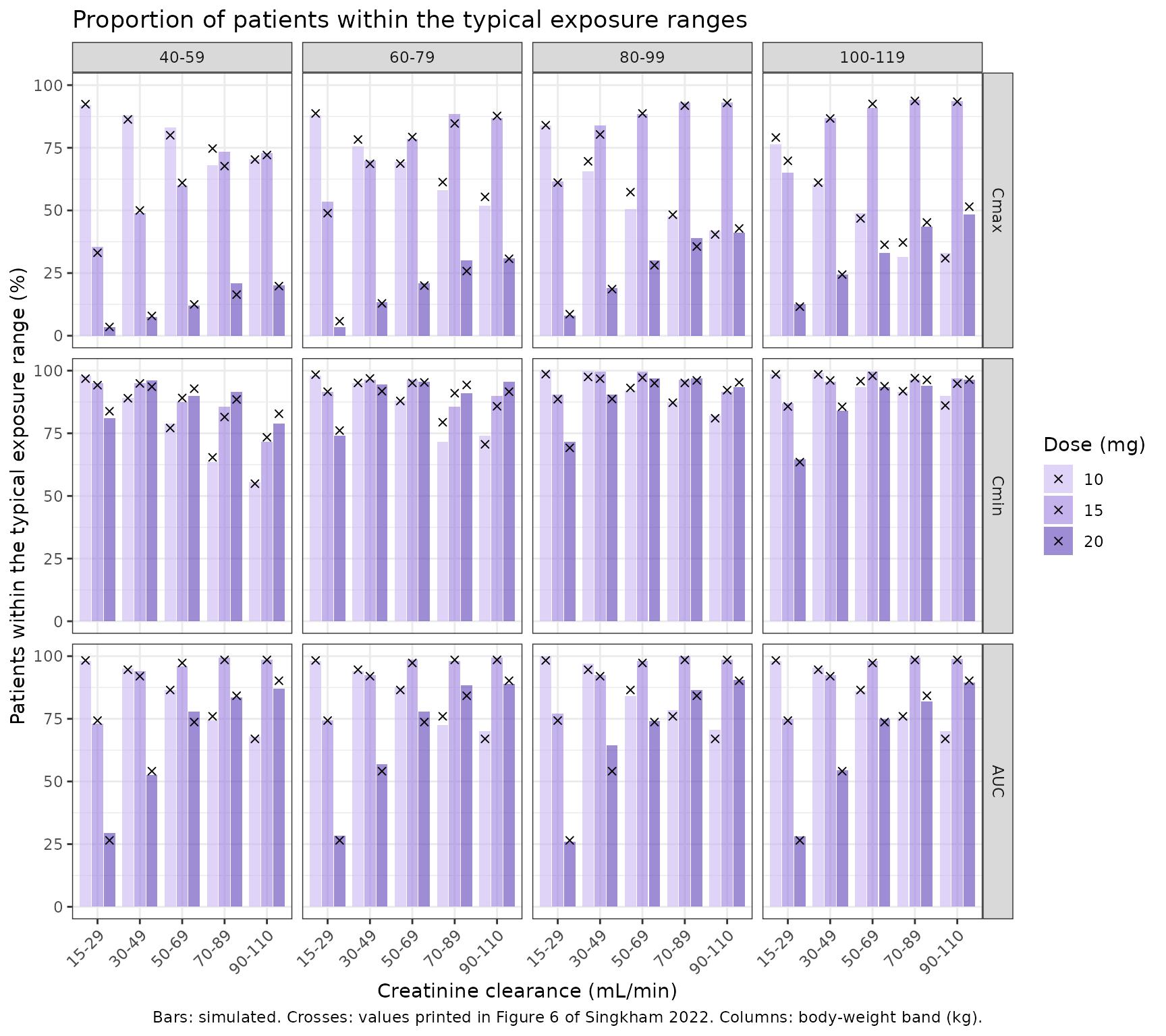
cmp6 |>
  group_by(metric) |>
  summarise(
    cells = n(),
    median_abs_diff = median(abs(diff)),
    p90_abs_diff = unname(quantile(abs(diff), 0.9)),
    max_abs_diff = max(abs(diff)),
    .groups = "drop"
  ) |>
  dplyr::rename(
    "Metric" = metric, "Cells" = cells,
    "Median |difference| (points)" = median_abs_diff,
    "90th pct |difference| (points)" = p90_abs_diff,
    "Max |difference| (points)" = max_abs_diff
  ) |>
  knitr::kable(digits = 1,
caption = "Simulated minus published percentage within range, by metric (percentage points).")| Metric | Cells | Median |difference| (points) | 90th pct |difference| (points) | Max |difference| (points) |
|---|---|---|---|---|
| Cmax | 60 | 1.3 | 4.6 | 6.8 |
| Cmin | 60 | 1.6 | 3.8 | 7.9 |
| AUC | 60 | 1.0 | 3.2 | 10.4 |
# With 200 patients per cell the Monte Carlo SE of a percentage is at most
# 3.5 points, so a correct model gives a median absolute difference near
# 2 points. A wrong omega scale (CV read as sqrt(omega^2)) or a wrong
# exponent shifts many cells by 5-20 points.
auc_cmp <- dplyr::filter(cmp6, metric == "AUC")
stopifnot(
  abs(median(auc_cmp$diff)) < 3,
  median(abs(auc_cmp$diff)) < 4,
  quantile(abs(auc_cmp$diff), 0.9) < 8,
  median(abs(cmp6$diff)) < 5,
  quantile(abs(cmp6$diff), 0.9) < 12
)
PKNCA validation
Figure 5 shows the simulated AUC0-24 distribution by CrCl band for each dose. The block below simulates 100 patients per dose and CrCl band (weight uniform over 40-120 kg, covering the four Figure 6 weight bands) to steady state and computes Cmax, Cmin and AUC0-24 over the tenth dosing interval with PKNCA.
n_per_arm <- 100L
subj5 <- tidyr::crossing(crcl_bands, dose_mg = c(10, 15, 20)) |>
  tidyr::uncount(n_per_arm) |>
  mutate(
    id = row_number(),
    CRCL = runif(n(), crcl_lo, crcl_hi),
    WT = runif(n(), 40, 120),
    treatment = paste0(dose_mg, " mg | CrCl ", crcl_band)
  ) |>
  select(id, treatment, dose_mg, crcl_band, CRCL, WT)

ev5 <- bind_rows(
  subj5 |> tidyr::crossing(time = seq(0, t_last, by = tau)) |>
    mutate(evid = 1L, amt = dose_mg, cmt = "depot"),
  subj5 |> tidyr::crossing(time = c(0, seq(t_last, t_last + tau, by = 0.5))) |>
    mutate(evid = 0L, amt = 0, cmt = "central")
) |>
  arrange(id, time, desc(evid))
stopifnot(!anyDuplicated(unique(ev5[, c("id", "time", "evid")])))

sim5 <- rxode2::rxSolve(mod, events = ev5, keep = c("treatment", "dose_mg", "crcl_band"),
                        returnType = "data.frame")
sim5 |>
  dplyr::filter(time == t_last) |>
  distinct(id, treatment, dose_mg, crcl_band) |>
  left_join(
    sim5 |>
      dplyr::filter(time >= t_last) |>
      group_by(id) |>
      summarise(auc = 1000 * sum(diff(time) * (head(Cc, -1) + tail(Cc, -1)) / 2)),
    by = "id"
  ) |>
  ggplot(aes(crcl_band, auc)) +
  geom_boxplot(outlier.shape = NA, fill = "#c9b6f2") +
  geom_hline(yintercept = c(1860, 5434), linetype = "dashed") +
  facet_wrap(~ paste0("Rivaroxaban ", dose_mg, " mg once daily")) +
  coord_cartesian(ylim = c(1000, 11000)) +
  labs(x = "Creatinine clearance (mL/min)", y = "AUC0-24 (ng*h/mL)",
       caption = "Replicates Figure 5 of Singkham 2022. Dashed lines: typical AUC0-24 range.") +
  theme_bw()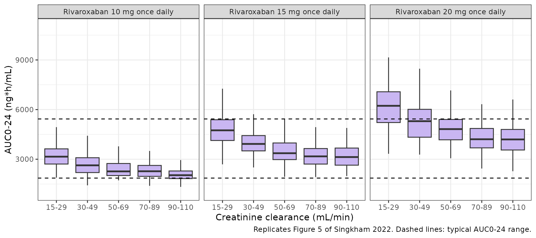
# Concentrations converted from mg/L (model units) to ng/mL, the unit of
# the paper's simulation figures.
sim_nca <- sim5 |>
  dplyr::filter(!is.na(Cc)) |>
  mutate(Cc = 1000 * Cc) |>
  select(id, time, Cc, treatment)
sim_nca <- bind_rows(
  sim_nca,
  sim_nca |> distinct(id, treatment) |> mutate(time = 0, Cc = 0)
) |>
  distinct(id, treatment, time, .keep_all = TRUE) |>
  arrange(id, treatment, time)

dose_df <- ev5 |>
  dplyr::filter(evid == 1) |>
  select(id, time, amt, treatment)

conc_obj <- PKNCA::PKNCAconc(sim_nca, Cc ~ time | treatment + id,
                             concu = "ng/mL", timeu = "h")
dose_obj <- PKNCA::PKNCAdose(dose_df, amt ~ time | treatment + id, doseu = "mg")
intervals <- data.frame(
  start = t_last, end = t_last + tau,
  cmax = TRUE, tmax = TRUE, cmin = TRUE, auclast = TRUE
)
nca_res <- PKNCA::pk.nca(PKNCA::PKNCAdata(conc_obj, dose_obj, intervals = intervals))
Comparison against Figure 5
The paper reports no NCA table; the reference values below are the Figure 5 medians digitised by the maintainers.
published <- fig5 |>
  mutate(treatment = paste0(dose, " mg | CrCl ", crcl_band)) |>
  select(treatment, auclast = fig5_median)

cmp <- nlmixr2lib::ncaComparisonTable(
  simulated = nca_res,
  reference = published,
  by = "treatment",
  params = "auclast",
  units = c(auclast = "ng*h/mL"),
  tolerance_pct = 20
)
knitr::kable(cmp, caption = "Simulated (PKNCA median) vs. Figure 5 median steady-state AUC0-24. * differs from reference by >20%.")| NCA parameter | treatment | Reference | Simulated | % diff |
|---|---|---|---|---|
| AUClast (ng*h/mL) | 10 mg | CrCl 15-29 | 3150 | 3150 | +0.2% |
| AUClast (ng*h/mL) | 10 mg | CrCl 30-49 | 2650 | 2630 | -0.7% |
| AUClast (ng*h/mL) | 10 mg | CrCl 50-69 | 2380 | 2270 | -4.8% |
| AUClast (ng*h/mL) | 10 mg | CrCl 70-89 | 2200 | 2270 | +3.3% |
| AUClast (ng*h/mL) | 10 mg | CrCl 90-110 | 2060 | 2030 | -1.2% |
| AUClast (ng*h/mL) | 15 mg | CrCl 15-29 | 4700 | 4750 | +1.0% |
| AUClast (ng*h/mL) | 15 mg | CrCl 30-49 | 4000 | 3920 | -1.9% |
| AUClast (ng*h/mL) | 15 mg | CrCl 50-69 | 3550 | 3360 | -5.3% |
| AUClast (ng*h/mL) | 15 mg | CrCl 70-89 | 3280 | 3170 | -3.3% |
| AUClast (ng*h/mL) | 15 mg | CrCl 90-110 | 3080 | 3130 | +1.6% |
| AUClast (ng*h/mL) | 20 mg | CrCl 15-29 | 6250 | 6230 | -0.4% |
| AUClast (ng*h/mL) | 20 mg | CrCl 30-49 | 5330 | 5300 | -0.6% |
| AUClast (ng*h/mL) | 20 mg | CrCl 50-69 | 4750 | 4820 | +1.5% |
| AUClast (ng*h/mL) | 20 mg | CrCl 70-89 | 4370 | 4210 | -3.7% |
| AUClast (ng*h/mL) | 20 mg | CrCl 90-110 | 4100 | 4200 | +2.3% |
nca_auc <- as.data.frame(nca_res) |>
  dplyr::filter(PPTESTCD == "auclast") |>
  group_by(treatment) |>
  summarise(sim_median = median(PPORRES), .groups = "drop") |>
  inner_join(published, by = "treatment") |>
  mutate(pct_diff = 100 * (sim_median - auclast) / auclast)
# Centre and robust envelope only (100 patients per arm).
stopifnot(
  nrow(nca_auc) == 15L,
  abs(median(nca_auc$pct_diff)) < 5,
  quantile(abs(nca_auc$pct_diff), 0.9) < 12
)
as.data.frame(nca_res) |>
  dplyr::filter(PPTESTCD %in% c("cmax", "cmin", "auclast", "tmax")) |>
  group_by(treatment, PPTESTCD) |>
  summarise(median = median(PPORRES), .groups = "drop") |>
  tidyr::pivot_wider(names_from = PPTESTCD, values_from = median) |>
  dplyr::rename(
    "Dose | CrCl band" = treatment,
    "Cmax (ng/mL)" = cmax, "Cmin (ng/mL)" = cmin,
    "AUC0-24 (ng*h/mL)" = auclast, "Tmax (h)" = tmax
  ) |>
knitr::kable(digits = 1, caption = "Median steady-state exposure by dose and CrCl band (PKNCA).")| Dose | CrCl band | AUC0-24 (ng*h/mL) | Cmax (ng/mL) | Cmin (ng/mL) | Tmax (h) |
|---|---|---|---|---|
| 10 mg | CrCl 15-29 | 3154.8 | 229.9 | 56.6 | 3.2 |
| 10 mg | CrCl 30-49 | 2631.1 | 207.4 | 33.5 | 3.0 |
| 10 mg | CrCl 50-69 | 2265.2 | 195.0 | 25.3 | 3.0 |
| 10 mg | CrCl 70-89 | 2272.7 | 193.7 | 26.6 | 2.5 |
| 10 mg | CrCl 90-110 | 2034.7 | 180.6 | 18.9 | 3.0 |
| 15 mg | CrCl 15-29 | 4746.5 | 347.1 | 78.3 | 3.0 |
| 15 mg | CrCl 30-49 | 3923.7 | 313.5 | 50.7 | 3.0 |
| 15 mg | CrCl 50-69 | 3363.1 | 288.2 | 36.5 | 3.2 |
| 15 mg | CrCl 70-89 | 3172.5 | 285.1 | 30.2 | 3.0 |
| 15 mg | CrCl 90-110 | 3130.5 | 289.7 | 30.9 | 3.0 |
| 20 mg | CrCl 15-29 | 6227.8 | 447.9 | 96.9 | 3.0 |
| 20 mg | CrCl 30-49 | 5298.6 | 420.1 | 63.8 | 3.0 |
| 20 mg | CrCl 50-69 | 4820.1 | 394.0 | 54.2 | 3.0 |
| 20 mg | CrCl 70-89 | 4206.7 | 367.8 | 40.9 | 3.0 |
| 20 mg | CrCl 90-110 | 4196.2 | 370.5 | 39.1 | 3.0 |
Assumptions and deviations
- Between-subject variability scale. Table 2 prints IIV as %CV. The model uses omega^2 = log(1 + CV^2). The Wald 95% intervals in Table 2 confirm this reading: back-transforming omega^2 x (1 +/- 1.96 x RSE) through CV = sqrt(exp(omega^2) - 1) reproduces the printed intervals to within 0.05 percentage points (16.66-26.25% vs printed 16.67-26.24% for CL/F; 66.37-85.14% vs 66.39-85.10% for ka), while the CV = sqrt(omega^2) reading misses by up to 2 points.
- Residual error. The additive RUV of 0.092 mg/L (92 ng/mL) carries concentration units in Table 2 and is treated as a standard deviation. It is large relative to trough concentrations; the paper’s Monte Carlo exposure metrics (and the reproductions here) use individual predictions without residual error.
- CrCl exponent. Table 2 and its footnote c give 0.277; the Results text quotes 0.278. The table value is used.
- Reference covariate values. CRCL is normalised to 57.5 mL/min and WT to 63 kg exactly as printed in the Table 2 footnotes. The paper does not state which cohort statistics these are (the cohort means are 59.0 mL/min and 64.0 kg).
- CRCL is raw Cockcroft-Gault mL/min, not BSA-normalised, as stated in Methods section 2.3.
-
ka prior. ka and its IIV were estimated under a
frequentist
$PRIORfrom an earlier Japanese population PK study (reference 23 of the paper). The packaged values are the reported posterior estimates (Table 2); the prior itself is not part of the model. - Figure 6 simulation design. The paper does not describe how CrCl and weight were distributed within each band; uniform distributions are assumed here. The Methods text lists the weight bands as “15-29, 30-59, 60-89, and 90-119 kg”, which conflicts with the figure panels (40-59, 60-79, 80-99, 100-119 kg); the panel labels are used. Cmin is the concentration at the end of the dosing interval.
- Figure 5 medians were digitised by the maintainers from the published boxplots (about +/- 50 ng*h/mL).
- No erratum was found for this article (Europe PMC search, 2026-10-05).