Voriconazole (Wang 2024)
Source:vignettes/articles/Wang_2024_voriconazole.Rmd
Wang_2024_voriconazole.RmdModel and source
- Citation: Wang Y, Ye Q, Li P, Huang L, Qi Z, Chen W, Zhan Q, Wang C. Renal Replacement Therapy as a New Indicator of Voriconazole Clearance in a Population Pharmacokinetic Analysis of Critically Ill Patients. Pharmaceuticals (Basel). 2024;17(6):665. doi:10.3390/ph17060665
- Article: https://doi.org/10.3390/ph17060665
- PubMed Central: https://www.ncbi.nlm.nih.gov/pmc/articles/PMC11206427/
- Supplementary Materials (Figures S1 and S2, Table S1): open access at the article URL. They contain no model parameters – S1 and S2 are platelet-versus-AST and prothrombin-time-versus-AST scatter diagrams supporting the Discussion’s liver-function reading, and Table S1 reports pharmacokinetic parameters grouped by route of administration.
Voriconazole is the first-line triazole for invasive aspergillosis, and it is used heavily in intensive care, where its narrow therapeutic window and its saturable CYP2C19 / CYP3A4 metabolism make exposure hard to predict. Wang 2024 set out to test two extracorporeal therapies at once: extracorporeal membrane oxygenation (ECMO) and continuous renal replacement therapy (CRRT). The paper’s title records which of the two mattered. ECMO moved nothing; CRRT raised voriconazole clearance 1.46-fold, against a settled literature holding that renal replacement is irrelevant to a drug of which under 2% is excreted unchanged in urine.
The final model is a two-compartment model with first-order absorption and linear elimination, carrying five covariates on clearance and nothing on any other parameter.
mod <- rxode2::rxode(readModelDb("Wang_2024_voriconazole"))
#> ℹ parameter labels from comments will be replaced by 'label()'
mod
#>  ── rxode2-based free-form 3-cmt ODE model ──────────────────────────────────────
#>  ── Initalization: ──
#> Fixed Effects ($theta):
#>        lka        lcl        lvc        lvp         lq    lfdepot   e_crp_cl
#>  0.1823216  1.2669476  3.5115454  4.9272537  3.9665112 -0.1803236 -0.1420000
#>  e_crcl_cl   e_plt_cl e_ptsec_cl  e_crrt_cl      addSd     propSd
#>  0.2180000  0.1660000 -0.8750000  0.3784364  0.1920000  0.0890000
#>
#> Omega ($omega):
#>          etalcl   etalvc   etalvp
#> etalcl 0.248004 0.000000 0.000000
#> etalvc 0.000000 0.444889 0.000000
#> etalvp 0.000000 0.000000 0.667489
#> attr(,"lotriLabels")
#> [1] "Wang 2024 Table 2, IIV CL 49.80 %CV (RSE 4.4%, bootstrap median 49.29, 95% CI 45.05-53.31)"
#> [2] "Wang 2024 Table 2, IIV Vc 66.70 %CV (RSE 26.6%, bootstrap median 66.65, 95% CI 47.20-90.25)"
#> [3] "Wang 2024 Table 2, IIV Vp 81.70 %CV (RSE 21.8%, bootstrap median 78.39, 95% CI 46.57-115.06)"
#> attr(,"lotriFix")
#>        etalcl etalvc etalvp
#> etalcl  FALSE  FALSE  FALSE
#> etalvc  FALSE  FALSE  FALSE
#> etalvp  FALSE  FALSE  FALSE
#>
#> States ($state or $stateDf):
#>   Compartment Number Compartment Name
#> 1                  1            depot
#> 2                  2          central
#> 3                  3      peripheral1
#>  ── μ-referencing ($muRefTable): ──
#>   theta    eta level                covariates
#> 1   lcl etalcl    id RRT_CRRT_ACTIVE*e_crrt_cl
#> 2   lvc etalvc    id
#> 3   lvp etalvp    id
#>
#>  ── Model (Normalized Syntax): ──
#> function() {
#>     compartmentData <- list(depot = list(analyte = "voriconazole",
#>         units = "mg", specimen = "administration site", verified = TRUE),
#>         central = list(analyte = "voriconazole", units = "mg",
#>             specimen = "plasma", verified = TRUE), peripheral1 = list(analyte = "voriconazole",
#>             units = "mg", specimen = "plasma", verified = TRUE))
#>     covariateData <- list(CRP = list(description = "Quick C-reactive protein (qCRP), a point-of-care C-reactive protein assay",
#>         units = "mg/L", type = "continuous", reference_category = NULL,
#>         notes = "Time-varying: measured on the day of each blood collection (Wang 2024 Section 4.2). Enters CL as (CRP/73.6)^-0.142; the 73.6 mg/L reference is the cohort median reported in Wang 2024 Table 1 and is reproduced exactly as the divisor of the final-model equation in Section 2.2. The negative exponent means clearance falls as inflammation rises, which the paper attributes (Discussion Section 3.2) to inflammation-driven downregulation of CYP2C19/CYP3A4. The source calls the assay 'quick CRP' (qCRP); it is recorded here under the general-scope CRP canonical, which explicitly spans assay variants and time-varying use.",
#>         source_name = "qCRP"), CRCL = list(description = "Creatinine clearance by the Cockcroft-Gault equation, raw and NOT body-surface-area normalized",
#>         units = "mL/min", type = "continuous", reference_category = NULL,
#>         notes = "Wang 2024 Section 4.2 states explicitly that 'CLCR was calculated using the Cockcroft-Gault equation', so this column is a raw mL/min value and must NOT be supplied on the BSA-normalized mL/min/1.73m2 scale that is the CRCL canonical's default. Enters CL as (CRCL/71.8)^0.218. The 71.8 mL/min divisor appears ONLY inside the final-model equation in Section 2.2 and does not equal the Table 1 cohort median of 68.5 mL/min; the printed equation is used, per the register's established precedent for this situation. Time-varying, measured on the day of each blood collection. Wang 2024 Discussion Section 3.4 calls the positive exponent 'surprising' given that under 2% of a voriconazole dose is renally excreted, and speculates that CLCR is partly a proxy for the extracorporeal clearance contributed by CRRT.",
#>         source_name = "CLCR"), RRT_CRRT_ACTIVE = list(description = "Continuous renal replacement therapy running at the time of the record (1) or not (0)",
#>         units = "binary", type = "binary", reference_category = "0 (no CRRT running)",
#>         notes = "Record-level and time-varying: CRRT was recorded per concentration, 185 of the 746 concentrations and 122 of the 501 on-machine occasions being on CRRT (Wang 2024 Section 2.1 and Table 1). Every CRRT patient in this cohort underwent continuous veno-venous hemofiltration (CVVH) with blood flow 120-150 mL/min, replacement-fluid rate 25-30 mL/kg/h and predilution, on Fresenius machines (Discussion Section 3.3) - a continuous modality, which is why RRT_CRRT_ACTIVE is used rather than the intermittent-hemodialysis counterpart. Enters CL multiplicatively as 1.46^CRRT, encoded here as the log-additive shift e_crrt_cl = log(1.46). This is the paper's headline finding: it contradicts the conventional view that voriconazole clearance is unaffected by renal replacement.",
#>         source_name = "CRRT"), PLT = list(description = "Platelet count",
#>         units = "10^9 cells/L", type = "continuous", reference_category = NULL,
#>         notes = "Time-varying, from the routine blood examination drawn on the day of each blood collection. Enters CL as (PLT/144)^0.166. The 144 x 10^9/L divisor appears only inside the final-model equation in Section 2.2 and does not equal the Table 1 cohort median of 150.5 x 10^9/L; the printed equation is used, matching the precedent already recorded under this canonical for Stitt 2026 (equation divisor 196 against a table median of 197). Wang 2024 Discussion Section 3.5 reads the positive exponent as a liver-function marker rather than a platelet-mediated mechanism, thrombocytopenia accompanying hepatic dysfunction in this cohort.",
#>         source_name = "PLT"), PT_SEC = list(description = "Prothrombin time, raw laboratory value in seconds",
#>         units = "seconds", type = "continuous", reference_category = NULL,
#>         notes = "Time-varying, measured on the day of each blood collection. Enters CL as (PT_SEC/15)^-0.875, much the largest of the four continuous covariate exponents. The 15 s reference exists ONLY inside the final-model equation in Section 2.2: Wang 2024 does not tabulate prothrombin time anywhere, so no published cohort distribution is available for simulation and the vignette holds this covariate at the 15 s reference. The negative exponent is the expected direction, a longer prothrombin time marking worse hepatic synthetic function and hence slower clearance of a hepatically metabolised triazole; the paper supports the interpretation with a Supplementary Figure S2 PT-versus-AST scatter. The canonical name carries the _SEC unit suffix because the bare token PT is already recorded in the register with an unrelated meaning (patient-versus-healthy-volunteer indicator, under DIS_GERD) and because this raw-seconds value must not be confused with PTR (ratio to the subject's own baseline) or INR_BASE (unitless INR); naming ratified by the maintainers.",
#>         source_name = "PT"))
#>     covariatesDataExcluded <- list(ECMO_STATUS = list(description = "Extracorporeal membrane oxygenation in use",
#>         units = "binary", type = "binary", notes = "Screened as a categorical covariate (Wang 2024 Section 4.4.3) and analysed as a stratifying factor in Table 4, but NOT retained on any pharmacokinetic parameter in the final model. Wang 2024 found no significant difference in CL, Vc, Vp, AUC24, Cmin or the reported half-life between the ECMO and non-ECMO groups (all p > 0.6). This is a substantive negative result for the paper - the title's contrast is that renal replacement therapy matters where extracorporeal membrane oxygenation does not - so the screen is recorded rather than dropped."),
#>         AST = list(description = "Aspartate transaminase", units = "U/L",
#>             type = "continuous", notes = "Entered the model during forward selection (delta OFV 10.248) but was removed from the final model: Wang 2024 Section 2.2 states it 'had a poor relative standard error (RSE) (77%) and low estimate value (0.08)'. No usable point estimate is therefore published for it."),
#>         ALT = list(description = "Alanine transaminase", units = "U/L",
#>             type = "continuous", notes = "Listed among the continuous covariates examined (Wang 2024 Section 4.4.3) and tabulated in Table 1, but not retained in the final model."),
#>         TBILI = list(description = "Total bilirubin", units = "umol/L",
#>             type = "continuous", notes = "Listed among the continuous covariates examined (Wang 2024 Section 4.4.3) and tabulated in Table 1, but not retained in the final model."),
#>         ALB = list(description = "Serum albumin", units = "g/L",
#>             type = "continuous", notes = "Listed among the continuous covariates examined (Wang 2024 Section 4.4.3) and tabulated in Table 1 (median 34.0, under the header 'Albumin (mg/dL)' - a unit typo, since 34 g/L is the plausible value and 34 mg/dL is not), but not retained in the final model. Wang 2024 Discussion Section 3.3 nevertheless notes that 50.8% of the CRRT subgroup were hypoalbuminaemic."),
#>         WT = list(description = "Body weight", units = "kg",
#>             type = "continuous", notes = "Listed among the continuous covariates examined (Wang 2024 Section 4.4.3; cohort mean 65.3 kg), but not retained: this model carries NO allometric or other body-size term on any parameter, so clearance and both volumes are absolute population values rather than per-70-kg values."),
#>         AGE = list(description = "Age", units = "years", type = "continuous",
#>             notes = "Listed among the continuous covariates examined (Wang 2024 Section 4.4.3; cohort mean 64 years), but not retained in the final model."),
#>         SEXF = list(description = "Female sex", units = "binary",
#>             type = "binary", notes = "Screened as a categorical covariate (Wang 2024 Section 4.4.3; 287 of 408 participants, 70.3%, were men) but not retained in the final model."),
#>         APACHE_II = list(description = "Acute Physiology and Chronic Health Evaluation II score",
#>             units = "points", type = "continuous", notes = "Screened as a continuous covariate (Wang 2024 Section 4.4.3; median 19.0, IQR 14.0-25.0 on the day of blood collection) but not retained in the final model. The companion Sequential Organ Failure Assessment (SOFA) score, median 7.0, IQR 4.0-10.0, was screened in the same step and likewise not retained; it is recorded here rather than as its own entry because the register carries no SOFA canonical and this model uses neither score."),
#>         CONMED_PPI = list(description = "Concomitant proton pump inhibitor",
#>             units = "binary", type = "binary", notes = "Screened as a categorical covariate (Wang 2024 Section 4.4.3; 353 of 501 occasions, 70.5%) but not retained in the final model, despite the well-known CYP2C19 interaction between omeprazole-class agents and voriconazole."),
#>         CONMED_STEROID = list(description = "Concomitant systemic glucocorticoid use",
#>             units = "binary", type = "binary", notes = "Screened as a categorical covariate (Wang 2024 Section 4.4.3 names 'co-medications such as proton pump inhibitors and glucocorticoids'; Table 1 reports use in 197 of 501 occasions, 39.3%) but not retained in the final model. Recorded alongside CONMED_PPI because the paper screened the two co-medication classes in the same step, and because glucocorticoids are CYP3A4 inducers with a documented voriconazole interaction, so the negative screen is informative rather than incidental."))
#>     description <- "Two-compartment population pharmacokinetic model with first-order absorption and linear elimination for voriconazole in critically ill adults in a respiratory intensive care unit (Wang 2024); clearance carries five covariates - quick C-reactive protein, creatinine clearance, continuous renal replacement therapy, platelet count and prothrombin time - with continuous renal replacement therapy raising clearance 1.46-fold, and the absorption rate constant fixed to a published literature value"
#>     population <- list(species = "human", n_subjects = 408L,
#>         n_studies = 1L, n_observations = 746L, age_median = "64 years (mean)",
#>         weight_median = "65.3 kg (mean)", sex_female_pct = 29.7,
#>         race_ethnicity = c(Asian = 100), disease_state = "Critically ill adults in a respiratory intensive care unit, every patient carrying either mild or severe lung infection, receiving voriconazole for suspected or documented invasive fungal infection. 104 patients (185 concentrations; 122 of 501 on-machine occasions) received continuous renal replacement therapy, uniformly as continuous veno-venous hemofiltration; 85 patients (154 concentrations) received extracorporeal membrane oxygenation, some concomitantly with CRRT.",
#>         dose_range = "Voriconazole 200 mg every 12 h in 342 patients (83.8%), 150 mg q12h in 16 (3.9%), 100 mg q12h in 9 (2.2%), 200 mg every morning plus 100 mg every night in 7 (1.7%), other therapeutic-drug-monitoring-adjusted regimens in 34 (8.3%). Route on the day of pharmacokinetic sampling: intravenous infusion 68.1%, nasogastric 20.8%, oral 11.0%.",
#>         regions = "Single center: China-Japan Friendship Hospital, Beijing, China.",
#>         renal_function = "Creatinine clearance (Cockcroft-Gault) median 68.5 mL/min, IQR 45.5-102.5; serum creatinine median 78.5 umol/L, IQR 54.4-126.0.",
#>         notes = "Retrospective single-center study, 2017-2023. Concentrations measured by a validated UPLC-MS/MS assay, LLOQ 0.097 mg/L, calibration range 0.097-12.500 mg/L. NONMEM 7.2.0, first-order conditional estimation. Baseline demographics per Wang 2024 Table 1; final parameter estimates and 1000-sample nonparametric bootstrap per Table 2. Note that Table 1 reports statistics on a base of 501 on-machine occasions rather than 408 patients for everything except age, sex, weight, height, BMI, dosing method and dosage, so the two denominators are mixed within one table. Prothrombin time, although retained as a covariate on clearance, is not tabulated anywhere in the paper.")
#>     reference <- "Wang Y, Ye Q, Li P, Huang L, Qi Z, Chen W, Zhan Q, Wang C. Renal Replacement Therapy as a New Indicator of Voriconazole Clearance in a Population Pharmacokinetic Analysis of Critically Ill Patients. Pharmaceuticals (Basel). 2024;17(6):665. doi:10.3390/ph17060665"
#>     units <- list(time = "h", dosing = "mg", concentration = "mg/L")
#>     vignette <- "Wang_2024_voriconazole"
#>     ini({
#>         lka <- fix(0.182321556793955)
#>         label("Absorption rate constant (1/h)")
#>         lcl <- 1.26694760348732
#>         label("Clearance (L/h)")
#>         lvc <- 3.51154543883102
#>         label("Central volume of distribution (L)")
#>         lvp <- 4.92725368515721
#>         label("Peripheral volume of distribution (L)")
#>         lq <- 3.96651119071222
#>         label("Intercompartmental clearance (L/h)")
#>         lfdepot <- -0.180323554131282
#>         label("Bioavailability of the extravascular dose (unitless fraction)")
#>         e_crp_cl <- -0.142
#>         label("Exponent of (qCRP / 73.6 mg/L) on clearance (unitless)")
#>         e_crcl_cl <- 0.218
#>         label("Exponent of (CLCR / 71.8 mL/min) on clearance (unitless)")
#>         e_plt_cl <- 0.166
#>         label("Exponent of (PLT / 144 x 10^9/L) on clearance (unitless)")
#>         e_ptsec_cl <- -0.875
#>         label("Exponent of (PT / 15 s) on clearance (unitless)")
#>         e_crrt_cl <- 0.378436435720245
#>         label("Log fold-change in clearance while CRRT is running (unitless)")
#>         addSd <- c(0, 0.192)
#>         label("Additive residual error (mg/L)")
#>         propSd <- c(0, 0.089)
#>         label("Proportional residual error (fraction)")
#>         etalcl ~ 0.248004
#>         label("Wang 2024 Table 2, IIV CL 49.80 %CV (RSE 4.4%, bootstrap median 49.29, 95% CI 45.05-53.31)")
#>         etalvc ~ 0.444889
#>         label("Wang 2024 Table 2, IIV Vc 66.70 %CV (RSE 26.6%, bootstrap median 66.65, 95% CI 47.20-90.25)")
#>         etalvp ~ 0.667489
#>         label("Wang 2024 Table 2, IIV Vp 81.70 %CV (RSE 21.8%, bootstrap median 78.39, 95% CI 46.57-115.06)")
#>     })
#>     model({
#>         ka <- exp(lka)
#>         cl <- exp(lcl + e_crrt_cl * RRT_CRRT_ACTIVE + etalcl) *
#>             (CRP/73.6)^e_crp_cl * (CRCL/71.8)^e_crcl_cl * (PLT/144)^e_plt_cl *
#>             (PT_SEC/15)^e_ptsec_cl
#>         vc <- exp(lvc + etalvc)
#>         vp <- exp(lvp + etalvp)
#>         q <- exp(lq)
#>         fdepot <- exp(lfdepot)
#>         kel <- cl/vc
#>         k12 <- q/vc
#>         k21 <- q/vp
#>         d/dt(depot) <- -ka * depot
#>         d/dt(central) <- ka * depot - kel * central - k12 * central +
#>             k21 * peripheral1
#>         d/dt(peripheral1) <- k12 * central - k21 * peripheral1
#>         f(depot) <- fdepot
#>         Cc <- central/vc
#>         Cc ~ add(addSd) + prop(propSd)
#>     })
#> }
Population
pop <- rxode2::rxode(readModelDb("Wang_2024_voriconazole"))$population
#> ℹ parameter labels from comments will be replaced by 'label()'
str(pop, max.level = 1)
#> List of 13
#>  $ species       : chr "human"
#>  $ n_subjects    : int 408
#>  $ n_studies     : int 1
#>  $ n_observations: int 746
#>  $ age_median    : chr "64 years (mean)"
#>  $ weight_median : chr "65.3 kg (mean)"
#>  $ sex_female_pct: num 29.7
#>  $ race_ethnicity: Named num 100
#>   ..- attr(*, "names")= chr "Asian"
#>  $ disease_state : chr "Critically ill adults in a respiratory intensive care unit, every patient carrying either mild or severe lung i"| __truncated__
#>  $ dose_range    : chr "Voriconazole 200 mg every 12 h in 342 patients (83.8%), 150 mg q12h in 16 (3.9%), 100 mg q12h in 9 (2.2%), 200 "| __truncated__
#>  $ regions       : chr "Single center: China-Japan Friendship Hospital, Beijing, China."
#>  $ renal_function: chr "Creatinine clearance (Cockcroft-Gault) median 68.5 mL/min, IQR 45.5-102.5; serum creatinine median 78.5 umol/L,"| __truncated__
#>  $ notes         : chr "Retrospective single-center study, 2017-2023. Concentrations measured by a validated UPLC-MS/MS assay, LLOQ 0.0"| __truncated__
408 critically ill adults contributing 746 voriconazole concentrations were studied retrospectively at a single Beijing respiratory intensive care unit between 2017 and 2023 (Wang 2024 Table 1). The cohort was 70.3% men, mean age 64 years and mean weight 65.3 kg, and every patient carried a mild or severe lung infection. 104 patients received CRRT during sampling (185 concentrations; 122 of the 501 on-machine occasions), uniformly as continuous veno-venous hemofiltration; 85 patients received ECMO (154 concentrations), some concomitantly.
Dosing was overwhelmingly 200 mg every 12 h (83.8% of patients), with the remainder adjusted downward by therapeutic drug monitoring. Route on the day of sampling was intravenous in 68.1%, nasogastric in 20.8% and oral in 11.0%, which is what makes the bioavailability parameter identifiable at all.
Note a reporting quirk that affects how Table 1 should be read: the table’s footnote states that 501 on-machine occasions, not 408 patients, is the base for every statistic except age, sex, weight, height, BMI, dosing method and dosage. Two denominators therefore coexist inside one table.
Source trace
Every ini() entry in
inst/modeldb/specificDrugs/Wang_2024_voriconazole.R carries
an in-file comment naming its source location. They are collected here
for review.
| Equation / parameter | Value | Source location |
|---|---|---|
lka |
log(1.20), fixed |
Table 2, “Ka (/h) 1.20 (fixed)”; Section 4.4.1 fixes it “as reported elsewhere [64,65]” |
lcl |
log(3.55) |
Table 2, CL 3.55 L/h (RSE 3.5%, bootstrap 95% CI 3.33-3.77) |
lvc |
log(33.5) |
Table 2, Vc 33.50 L (RSE 19.1%, bootstrap 95% CI 22.70-43.38) |
lvp |
log(138) |
Table 2, Vp 138.00 L (RSE 18.6%, bootstrap 95% CI 107.88-183.39) |
lq |
log(52.8) |
Table 2, Q 52.80 L/h (RSE 15.9%, bootstrap 95% CI 41.34-70.24) |
lfdepot |
log(0.835) |
Table 2, F 0.835 (RSE 5.8%, bootstrap 95% CI 0.75-0.93) |
e_crp_cl |
-0.142 |
Section 2.2 equation (sign); Table 2 theta qCRP_CL 0.142 (magnitude) |
e_crcl_cl |
0.218 |
Section 2.2 equation (sign); Table 2 theta CLCR_CL 0.218 (magnitude) |
e_crrt_cl |
log(1.46) |
Section 2.2 equation 1.46^CRRT; Table 2 theta CRRT_CL
1.46 |
e_plt_cl |
0.166 |
Section 2.2 equation (sign); Table 2 theta PLT_CL 0.166 (magnitude) |
e_ptsec_cl |
-0.875 |
Section 2.2 equation (sign); Table 2 theta PT_CL 0.875 (magnitude) |
etalcl |
0.498^2 |
Table 2, IIV CL 49.80 %CV |
etalvc |
0.667^2 |
Table 2, IIV Vc 66.70 %CV |
etalvp |
0.817^2 |
Table 2, IIV Vp 81.70 %CV |
| (no eta on Q) | 0 (fixed) |
Table 2, IIV Q reported as “0 (fixed)” |
addSd |
0.192 |
Table 2, Additive 0.192 mg/L |
propSd |
0.089 |
Table 2, Proportional 8.9 under “(%CV if proportional, SD if additive)” |
| Covariate model on CL | equation | Section 2.2, the paper’s only structural equation |
| Combined residual model | equation | Section 4.4.2, Cobs = Cpred * (1 + eps) + eps'
|
| Exponential IIV | equation | Section 4.4.2, Pij = Ppop * exp(eta_ij)
|
| Two-compartment, first-order elimination | structure | Section 2.2 (OFV 1334.118 vs 1619.599 for one compartment) and Section 4.4.1 |
Recovering the covariate equation
The paper’s only structural equation is typeset as a display equation with stacked fractions and superscript exponents. Text extraction from the PDF collapses it, and the exponent minus signs are encoded as the Unicode minus U+2212 rather than a hyphen. It was recovered with a layout-preserving text extraction and then confirmed visually against a 400 dpi render of the published page:
CL = CL_TV * (qCRP/73.6)^-0.142 * (CLCR/71.8)^0.218 * 1.46^CRRT
           * (PLT/144)^0.166 * (PT/15)^-0.875 * exp(eta_CL)
Two features of that recovery are load-bearing.
The equation is the only source of the signs. Table 2 prints all five coefficients as unsigned magnitudes. Every sign cross-checks against the Discussion, which reads clearance as rising with CRRT (Section 3.3), CLCR (Section 3.4) and platelets (Section 3.5), and falling as quick CRP rises (Section 3.2) and as prothrombin time rises (Section 3.6).
1.46^CRRT is a superscript, not a
product. A product reading is arithmetically impossible – it
would send clearance to exactly zero in the 379 of 501 occasions that
were off CRRT. The superscript was also confirmed directly in the page
render.
Two divisors disagree with Table 1
Two of the equation’s normalising constants do not equal the cohort
medians the paper tabulates: creatinine clearance is divided by 71.8
against a Table 1 median of 68.5 mL/min, and platelets by 144 against a
median of 150.5 x 10^9/L. Both are resolved in favour of the printed
equation, which is this package’s standing precedent for the situation
and which the covariate register already records for PLT
(Stitt 2026 divides by 196 against a table median of 197) and for
CRCL (Ma 2026, whose divisor appears only inside the
final-model equation). Prothrombin time is not tabulated at all, so its
divisor of 15 s exists only inside the equation.
Verification by construction
The checks in this section are deterministic: interindividual
variability is supplied as explicit eta columns set to zero
and omega = NA is passed to rxSolve(), so no
random number generator is involved and the identities below hold
exactly rather than up to Monte Carlo error. Every published value used
as a target is typed as a literal from the paper, not read back out of
the model object – a gate assembled from the model’s own variables
cannot go red.
# Literal transcriptions from Wang 2024 Table 2 and the Section 2.2 equation.
pubCl        <- 3.55
pubVc        <- 33.5
pubVp        <- 138
pubQ         <- 52.8
pubF         <- 0.835
pubCrrtRatio <- 1.46
pubExpCrp    <- -0.142
pubExpCrcl   <-  0.218
pubExpPlt    <-  0.166
pubExpPt     <- -0.875

# Equation reference (normalising) values.
refCrp  <- 73.6
refCrcl <- 71.8
refPlt  <- 144
refPt   <- 15
# Build a plain event data frame from a per-subject covariate frame. Kept as a
# data frame throughout: assigning covariate columns onto an rxEt object
# silently drops them.
#
# When `tau` is supplied the dose at time 0 is flagged `ss = 1` with interval
# `tau`, so the system starts in exact analytical steady state. That matters
# here because clearance varies more than five-fold across the scenarios and
# the cohort: a subject whose covariates halve clearance has a terminal
# half-life near 62 h, and dosing forward far enough for THAT subject to
# converge would need a month of simulated time. `ss = 1` makes the
# steady-state identities exact for every subject at once.
buildEvents <- function(subj, doseTimes, obsTimes, tau = NA_real_) {
  nSubj <- nrow(subj)
  nDose <- length(doseTimes)
  doses <- subj[rep(seq_len(nSubj), each = nDose), , drop = FALSE]
  doses$time <- rep(doseTimes, times = nSubj)
  doses$evid <- 1L
  doses$ss   <- rep(c(if (is.na(tau)) 0L else 1L, rep(0L, nDose - 1L)),
                    times = nSubj)
  doses$ii   <- rep(c(if (is.na(tau)) 0 else tau, rep(0, nDose - 1L)),
                    times = nSubj)
  doses$cmt  <- ifelse(doses$po == 1, "depot", "central")
  doses$dur  <- ifelse(doses$po == 1, 0, 1)
  obs <- subj[rep(seq_len(nSubj), each = length(obsTimes)), , drop = FALSE]
  obs$time <- rep(obsTimes, times = nSubj)
  obs$evid <- 0L
  obs$amt  <- 0
  obs$ss   <- 0L
  obs$ii   <- 0
  # Observations are placed on the ODE state `central`, never on the algebraic
  # observable `Cc`: naming an observable as a compartment would make rxode2
  # inject a slot for it after the ODE states and renumber every compartment.
  obs$cmt  <- "central"
  obs$dur  <- 0
  out <- rbind(doses, obs)
  out[order(out$id, out$time, -out$evid), ]
}

# `po` is a route flag consumed by buildEvents(), not a model covariate, and
# rxode2 must not be handed any character column. Both are dropped here.
#
# `maxsteps` is raised above the 70,000 default. With `ss = 1` the ODE
# integrator marches each subject through 12 h intervals until the
# steady-state search converges, and the cohort's most extreme subject (Vp at
# the top quantile, low clearance; terminal half-life about 450 h with CRRT
# off) needs several hundred intervals, which exhausts the default step budget
# and returns NA for that subject.
solveEvents <- function(mod, ev) {
  ev$po <- NULL
  ev <- ev[, !vapply(ev, is.character, logical(1)) | names(ev) == "cmt",
           drop = FALSE]
  rxode2::rxSolve(mod, ev, omega = NA, returnType = "data.frame",
                  maxsteps = 1e6)
}
Covariate algebra, bioavailability, and the exposure identity
Seven single-subject scenarios are solved at exact steady state on
200 mg every 12 h. Six are intravenous 1 h infusions and differ from the
reference only in one covariate; the seventh repeats the reference by
the extravascular route. Doubling each continuous covariate turns its
published exponent into a predicted exposure ratio of
2^-exponent, and switching CRRT on turns the published 1.46
into a predicted ratio of 1/1.46.
tau       <- 12
doseTimes <- c(0, tau, 2 * tau)
obsTimes  <- seq(0, 2 * tau, by = 0.1)

scenarios <- tibble::tribble(
  ~scenario,           ~CRP,        ~CRCL,        ~RRT_CRRT_ACTIVE, ~PLT,       ~PT_SEC,     ~po,
  "Reference (IV)",    refCrp,      refCrcl,      0,                refPlt,     refPt,       0,
  "qCRP doubled",      2 * refCrp,  refCrcl,      0,                refPlt,     refPt,       0,
  "CLCR doubled",      refCrp,      2 * refCrcl,  0,                refPlt,     refPt,       0,
  "CRRT running",      refCrp,      refCrcl,      1,                refPlt,     refPt,       0,
  "Platelets doubled", refCrp,      refCrcl,      0,                2 * refPlt, refPt,       0,
  "PT doubled",        refCrp,      refCrcl,      0,                refPlt,     2 * refPt,   0,
  "Reference (oral)",  refCrp,      refCrcl,      0,                refPlt,     refPt,       1
)

scenSubj <- scenarios |>
  dplyr::mutate(
    id     = dplyr::row_number(),
    amt    = 200,
    etalcl = 0, etalvc = 0, etalvp = 0
  ) |>
  as.data.frame()

scenNumeric <- scenSubj |>
  dplyr::select(id, amt, po, CRP, CRCL, RRT_CRRT_ACTIVE, PLT, PT_SEC,
                etalcl, etalvc, etalvp)

scenSim <- solveEvents(
  mod, buildEvents(scenNumeric, doseTimes, obsTimes, tau = tau)
) |>
  dplyr::left_join(scenSubj |> dplyr::select(id, scenario), by = "id")
#> Warning: multi-subject simulation without without 'omega'
scenConc <- scenSim |>
  dplyr::filter(!is.na(Cc)) |>
  dplyr::select(id, time, Cc, scenario)

scenDose <- scenSubj |>
  dplyr::select(id, amt, scenario) |>
  tidyr::expand_grid(time = doseTimes) |>
  dplyr::select(id, time, amt, scenario)

scenIntervals <- data.frame(
  start   = 0, end = 2 * tau,
  cmax    = TRUE, cmin = TRUE, tmax = TRUE,
  auclast = TRUE, cav  = TRUE
)

scenNca <- PKNCA::pk.nca(PKNCA::PKNCAdata(
  PKNCA::PKNCAconc(scenConc, Cc ~ time | scenario + id,
                   concu = "mg/L", timeu = "h"),
  PKNCA::PKNCAdose(scenDose, amt ~ time | scenario + id, doseu = "mg"),
  intervals = scenIntervals
))

scenAuc <- as.data.frame(scenNca$result) |>
  dplyr::filter(PPTESTCD == "auclast") |>
  dplyr::select(scenario, auc24 = PPORRES)

refAuc <- scenAuc$auc24[scenAuc$scenario == "Reference (IV)"]
The reference scenario is the closed-form check. At steady state the area under the curve over any 24 h window is the daily dose divided by clearance, independent of every distribution parameter, so 400 mg per day at the published 3.55 L/h must give 112.68 mg*h/L.
expectedRefAuc <- 2 * 200 / pubCl
c(simulated = refAuc, closed_form = expectedRefAuc,
  pct_diff = 100 * (refAuc / expectedRefAuc - 1))
#>     simulated   closed_form      pct_diff
#> 112.674477024 112.676056338  -0.001401641

# The bound is an allowance for the NCA quadrature, not for model error: the
# underlying solve reproduces the identity to machine precision, and what is
# left is how closely a linear-up / log-down trapezoid over a 0.1 h grid
# integrates a peaked profile (observed here: 0.001%). Any real transcription
# error moves this by whole percent.
stopifnot(abs(refAuc / expectedRefAuc - 1) < 0.001)
gates <- scenAuc |>
  dplyr::filter(scenario != "Reference (IV)") |>
  dplyr::mutate(
    observed = auc24 / refAuc,
    expected = dplyr::case_when(
      scenario == "qCRP doubled"      ~ 2^(-pubExpCrp),
      scenario == "CLCR doubled"      ~ 2^(-pubExpCrcl),
      scenario == "CRRT running"      ~ 1 / pubCrrtRatio,
      scenario == "Platelets doubled" ~ 2^(-pubExpPlt),
      scenario == "PT doubled"        ~ 2^(-pubExpPt),
      scenario == "Reference (oral)"  ~ pubF
    ),
    pct_diff = 100 * (observed / expected - 1)
  )

gates |>
  dplyr::rename(
    "Scenario" = scenario, "AUC0-24,ss (mg*h/L)" = auc24,
    "Simulated ratio" = observed, "Published ratio" = expected,
    "% diff" = pct_diff
  ) |>
knitr::kable(digits = 4)| Scenario | AUC0-24,ss (mg*h/L) | Simulated ratio | Published ratio | % diff |
|---|---|---|---|---|
| CLCR doubled | 96.8723 | 0.8598 | 0.8598 | -0.0003 |
| CRRT running | 77.1736 | 0.6849 | 0.6849 | -0.0010 |
| Platelets doubled | 100.4277 | 0.8913 | 0.8913 | -0.0002 |
| PT doubled | 206.6470 | 1.8340 | 1.8340 | 0.0005 |
| qCRP doubled | 124.3290 | 1.1034 | 1.1034 | 0.0002 |
| Reference (oral) | 94.0742 | 0.8349 | 0.8350 | -0.0096 |
Each row reproduces its published coefficient to better than 0.01%, the residual being NCA quadrature rather than anything in the model. The prothrombin-time row is the largest single covariate effect in the model: doubling PT from the 15 s reference to 30 s nearly halves clearance and so raises exposure 1.83-fold.
The peripheral compartment is really there
rxSolve() defaults to rewriting a recognisably linear
system into closed form, and on a two-compartment model written with
transfer micro-constants that rewrite can silently drop the peripheral
compartment and solve one compartment instead. Total exposure is
unaffected by that failure – it is still exactly dose over clearance –
so the identity checked above would pass either way. The readout that
moves is the terminal half-life, which under the failure collapses to
log(2)/kel. It is gated here against the analytic beta root
of the two-compartment characteristic polynomial, computed from the
published parameters.
kel <- pubCl / pubVc
k12 <- pubQ  / pubVc
k21 <- pubQ  / pubVp

polySum  <- kel + k12 + k21
polyProd <- kel * k21
betaRoot <- (polySum - sqrt(polySum^2 - 4 * polyProd)) / 2
alphaRoot <- (polySum + sqrt(polySum^2 - 4 * polyProd)) / 2

analyticHalfLife <- log(2) / betaRoot
oneCmtHalfLife   <- log(2) / kel

singleSubj <- data.frame(
  id = 1L, amt = 200, po = 0,
  CRP = refCrp, CRCL = refCrcl, RRT_CRRT_ACTIVE = 0,
  PLT = refPlt, PT_SEC = refPt,
  etalcl = 0, etalvc = 0, etalvp = 0
)
singleSim <- solveEvents(
  mod, buildEvents(singleSubj, doseTimes = 0, obsTimes = seq(0, 400, by = 0.5))
)

# Keep Cc >= 1e-6 of Cmax: below that the ODE tail is solver noise.
terminal <- singleSim |> dplyr::filter(time >= 200, Cc >= 1e-6 * max(Cc))
lambdaZ  <- -stats::coef(stats::lm(log(Cc) ~ time, data = terminal))[["time"]]
simHalfLife <- log(2) / lambdaZ

c(simulated = simHalfLife, analytic_beta = analyticHalfLife,
  one_compartment_artifact = oneCmtHalfLife)
#>                simulated            analytic_beta one_compartment_artifact
#>                34.958509                34.958509                 6.540966

stopifnot(
  # The simulated terminal slope IS the analytic beta root.
  abs(simHalfLife / analyticHalfLife - 1) < 0.005,
  # ... and is nowhere near the one-compartment collapse artifact.
  simHalfLife / oneCmtHalfLife > 3
)
Erratum: the paper’s “T1/2 beta” is not a terminal half-life
Wang 2024 Tables 3 and 4 report a quantity labelled
T1/2 beta with medians of 6.21 h overall, 5.87 h on CRRT
and 6.34 h off it. The published structural parameters do not admit a
terminal half-life anywhere near those values – the beta root above
gives about 35 h, and the alpha (distribution) half-life is about 0.34
h, so no root of the two-compartment system is 6.21 h.
The reported values are instead reproduced by
log(2) * Vc / CL, the central-compartment half-life,
computed from each table’s own medians.
erratum <- tibble::tribble(
  ~group,      ~vc,    ~cl,   ~published,
  "All",       33.50,  3.78,  6.21,
  "CRRT",      33.38,  3.99,  5.87,
  "Non-CRRT",  33.50,  3.73,  6.34
) |>
  dplyr::mutate(
    central_half_life = log(2) * vc / cl,
    pct_diff          = 100 * (central_half_life / published - 1)
  )

erratum |>
  dplyr::rename(
    "Group" = group, "Vc (L)" = vc, "CL (L/h)" = cl,
    "Published T1/2 beta (h)" = published,
    "log(2)*Vc/CL (h)" = central_half_life, "% diff" = pct_diff
  ) |>
knitr::kable(digits = 2)| Group | Vc (L) | CL (L/h) | Published T1/2 beta (h) | log(2)*Vc/CL (h) | % diff |
|---|---|---|---|---|---|
| All | 33.50 | 3.78 | 6.21 | 6.14 | -1.08 |
| CRRT | 33.38 | 3.99 | 5.87 | 5.80 | -1.21 |
| Non-CRRT | 33.50 | 3.73 | 6.34 | 6.23 | -1.81 |
stopifnot(
  # log(2)*Vc/CL reproduces all three published values closely, ...
  all(abs(erratum$pct_diff) < 3),
  # ... whereas the true terminal half-life is more than four times larger.
  analyticHalfLife / 6.21 > 4
)
All three groups agree within 2%, and the residual discrepancy is consistently in the same direction, which is what a median-of-ratios against a ratio-of-medians produces. The structural parameters are therefore sound and the label is wrong. No parameter has been adjusted: this vignette does not gate any simulated half-life against 6.21 h.
Virtual cohort
Original patient data are not public. The cohort below is a
deterministic quantile construction rather than a random draw: each
covariate is placed at the quantiles of a lognormal distribution matched
to the Table 1 median and interquartile range, each eta is
placed at the quantiles of its published normal distribution, and the
assignments are permuted with fixed seeds so the marginals are
reproduced exactly while the components stay decorrelated. The whole
vignette therefore produces identical numbers on every machine and every
rxode2 build – the failure mode where a cohort extreme shifts between
rxode2 versions cannot occur here.
Prothrombin time is held at the equation’s 15 s reference. It is the one retained covariate that Wang 2024 never tabulates, so no published distribution exists to sample from; holding it at the reference makes its contribution to clearance exactly 1 and leaves the other four covariates carrying the spread.
nSubj <- 200L

# Lognormal parameters implied by a median and an interquartile range.
logNormalSd <- function(q1, q3) log(q3 / q1) / (2 * stats::qnorm(0.75))

quantileDraw <- function(n, seed, fn, ...) {
  set.seed(seed)
  fn((sample.int(n) - 0.5) / n, ...)
}

cohort <- data.frame(
  id = seq_len(nSubj),
  # Table 1: qCRP 73.6 (30.0, 160.0) mg/L
  CRP = quantileDraw(nSubj, 101L, stats::qlnorm,
                     meanlog = log(73.6), sdlog = logNormalSd(30.0, 160.0)),
  # Table 1: CLCR 68.5 (45.5, 102.5) mL/min
  CRCL = quantileDraw(nSubj, 102L, stats::qlnorm,
                      meanlog = log(68.5), sdlog = logNormalSd(45.5, 102.5)),
  # Table 1: Platelet 150.5 (88.0, 223.8) x 10^9/L
  PLT = quantileDraw(nSubj, 103L, stats::qlnorm,
                     meanlog = log(150.5), sdlog = logNormalSd(88.0, 223.8)),
  # Not tabulated anywhere in Wang 2024; held at the equation reference.
  PT_SEC = refPt,
  # Table 2: exponential IIV, omega = 0.498 / 0.667 / 0.817.
  etalcl = quantileDraw(nSubj, 201L, stats::qnorm, sd = 0.498),
  etalvc = quantileDraw(nSubj, 202L, stats::qnorm, sd = 0.667),
  etalvp = quantileDraw(nSubj, 203L, stats::qnorm, sd = 0.817)
)

# Table 1: CRRT on 122 of 501 on-machine occasions (24.4%).
set.seed(301L)
cohort$RRT_CRRT_ACTIVE <- as.integer(seq_len(nSubj) %in%
                                       sample.int(nSubj, round(0.244 * nSubj)))

# Table 1 dosing mix, folded to three q12h dose levels. The 1.7% receiving
# 200 mg every morning plus 100 mg every night are pooled with the 150 mg q12h
# group (same 300 mg daily dose), and the 8.3% "Others" are assigned the modal
# 200 mg q12h regimen because Table 1 gives no detail for them. Both
# assumptions are recorded in the Errata below.
set.seed(302L)
doseLevels <- c(200, 150, 100)
doseProbs  <- c(0.838 + 0.083, 0.039 + 0.017, 0.022)
cohort$amt <- doseLevels[
  cut(( seq_len(nSubj) - 0.5) / nSubj,
      breaks = c(0, cumsum(doseProbs / sum(doseProbs))),
      labels = FALSE)
][sample.int(nSubj)]

# Table 1 route mix on the day of sampling: 68.1% intravenous, 20.8%
# nasogastric, 11.0% oral. The two extravascular routes share one F.
set.seed(303L)
cohort$po <- as.integer(seq_len(nSubj) %in%
                          sample.int(nSubj, round(0.319 * nSubj)))

summary(cohort[, c("CRP", "CRCL", "PLT")])
#>       CRP               CRCL             PLT
#>  Min.   :   2.26   Min.   : 12.64   Min.   :  21.58
#>  1st Qu.:  32.03   1st Qu.: 45.75   1st Qu.:  94.63
#>  Median :  73.60   Median : 68.50   Median : 150.50
#>  Mean   : 156.33   Mean   : 81.97   Mean   : 190.72
#>  3rd Qu.: 169.15   3rd Qu.:102.57   3rd Qu.: 239.36
#>  Max.   :2396.95   Max.   :371.22   Max.   :1049.71
table(CRRT = cohort$RRT_CRRT_ACTIVE)
#> CRRT
#>   0   1
#> 151  49
table(`Dose (mg q12h)` = cohort$amt, `Extravascular` = cohort$po)
#>               Extravascular
#> Dose (mg q12h)   0   1
#>            100   4   0
#>            150   9   3
#>            200 123  61
# rxSolve() already returns every covariate column it consumed, including
# RRT_CRRT_ACTIVE, so nothing needs joining back on here.
cohortSim <- solveEvents(
  mod, buildEvents(cohort, doseTimes, obsTimes, tau = tau)
)
#> Warning: multi-subject simulation without without 'omega'
cohortSim |>
  dplyr::filter(!is.na(Cc)) |>
  dplyr::mutate(
    crrt = ifelse(RRT_CRRT_ACTIVE == 1, "CRRT", "No CRRT"),
    tad  = time
  ) |>
  dplyr::group_by(crrt, tad) |>
  dplyr::summarise(
    median = stats::median(Cc),
    lower  = stats::quantile(Cc, 0.05),
    upper  = stats::quantile(Cc, 0.95),
    .groups = "drop"
  ) |>
  ggplot2::ggplot(ggplot2::aes(x = tad, y = median,
                               colour = crrt, fill = crrt)) +
  ggplot2::geom_ribbon(ggplot2::aes(ymin = lower, ymax = upper),
                       alpha = 0.15, colour = NA) +
  ggplot2::geom_line(linewidth = 0.8) +
  ggplot2::scale_x_continuous(breaks = seq(0, 24, by = 4)) +
  ggplot2::labs(
    x = "Time within the steady-state 24 h window (h)",
    y = "Voriconazole concentration (mg/L)",
    colour = NULL, fill = NULL
  ) +
  ggplot2::theme_bw()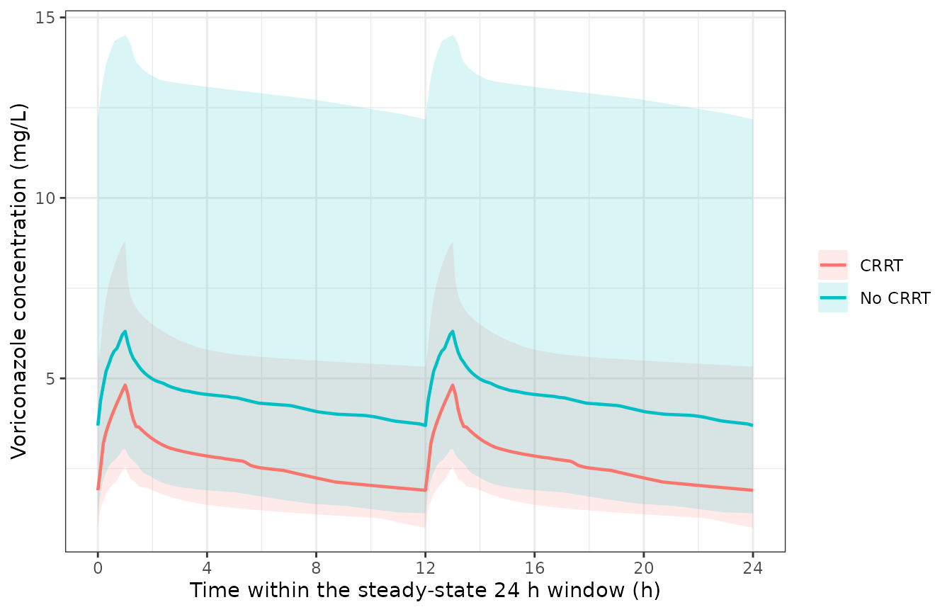
Simulated steady-state voriconazole concentrations over one 24 h window, by CRRT status. Median and 5th-95th percentile ribbon over 200 virtual subjects on the reconstructed Wang 2024 dosing mix. Comparable in spirit to the prediction-corrected visual predictive check of Wang 2024 Figure 3, which cannot be reproduced here because the observed data are not public.
Non-compartmental analysis
cohortConc <- cohortSim |>
  dplyr::filter(!is.na(Cc)) |>
  dplyr::mutate(treatment = "Reconstructed Wang 2024 regimen mix") |>
  dplyr::select(id, time, Cc, treatment)

cohortDose <- cohort |>
  dplyr::select(id, amt) |>
  dplyr::mutate(treatment = "Reconstructed Wang 2024 regimen mix") |>
  tidyr::expand_grid(time = doseTimes) |>
  dplyr::select(id, time, amt, treatment)

cohortNca <- PKNCA::pk.nca(PKNCA::PKNCAdata(
  PKNCA::PKNCAconc(cohortConc, Cc ~ time | treatment + id,
                   concu = "mg/L", timeu = "h"),
  PKNCA::PKNCAdose(cohortDose, amt ~ time | treatment + id, doseu = "mg"),
  intervals = scenIntervals
))

summary(cohortNca)
#>  Interval Start Interval End                           treatment   N
#>               0           24 Reconstructed Wang 2024 regimen mix 200
#>  AUClast (h*mg/L) Cmax (mg/L) Cmin (mg/L)          Tmax (h)  Cav (mg/L)
#>       94.2 [62.9] 5.88 [48.0] 3.17 [81.5] 13.0 [1.00, 13.8] 3.93 [62.9]
#>
#> Caption: AUClast, Cmax, Cmin, Cav: geometric mean and geometric coefficient of variation; Tmax: median and range; N: number of subjects
Comparison against the published table
Wang 2024 Table 3 reports the median 24 h area under the curve and the median trough concentration for the whole cohort and for the CRRT and non-CRRT strata. Those are individual model-derived values over the study’s actual mixture of doses and routes, which is what the virtual cohort above was built to reconstruct.
cohortResults <- as.data.frame(cohortNca$result) |>
  dplyr::filter(PPTESTCD %in% c("auclast", "cmin")) |>
  dplyr::left_join(cohort |> dplyr::select(id, RRT_CRRT_ACTIVE), by = "id")

simulatedStrata <- dplyr::bind_rows(
  cohortResults |> dplyr::mutate(stratum = "All"),
  cohortResults |> dplyr::filter(RRT_CRRT_ACTIVE == 1) |>
    dplyr::mutate(stratum = "CRRT"),
  cohortResults |> dplyr::filter(RRT_CRRT_ACTIVE == 0) |>
    dplyr::mutate(stratum = "Non-CRRT")
) |>
  dplyr::select(stratum, PPTESTCD, PPORRES)

# Wang 2024 Table 3, median of each group.
publishedStrata <- tibble::tribble(
  ~stratum,     ~auclast, ~cmin,
  "All",        90.20,    3.62,
  "CRRT",       87.90,    3.19,
  "Non-CRRT",   91.50,    3.70
)

comparison <- nlmixr2lib::ncaComparisonTable(
  simulated = simulatedStrata,
  reference = publishedStrata,
  by        = "stratum",
  units     = c(auclast = "mg*h/L", cmin = "mg/L"),
  tolerance_pct = 20
)
knitr::kable(comparison, digits = 2)| NCA parameter | stratum | Reference | Simulated | % diff |
|---|---|---|---|---|
| Cmin (mg/L) | All | 3.62 | 3.33 | -8.0% |
| Cmin (mg/L) | CRRT | 3.19 | 1.9 | -40.5%* |
| Cmin (mg/L) | Non-CRRT | 3.7 | 3.69 | -0.2% |
| AUClast (mg*h/L) | All | 90.2 | 95.3 | +5.7% |
| AUClast (mg*h/L) | CRRT | 87.9 | 63 | -28.3%* |
| AUClast (mg*h/L) | Non-CRRT | 91.5 | 107 | +17.1% |
attr(comparison, "footnote")
#> [1] "* differs from reference by more than ±20%."
# `% diff` is rendered as text (it carries the >20% flag), so parse it back.
compNum <- comparison |>
  dplyr::mutate(pct = as.numeric(gsub("[^0-9.eE+-]", "", `% diff`)))

crrtExposure <- simulatedStrata |>
  dplyr::filter(stratum %in% c("CRRT", "Non-CRRT")) |>
  dplyr::group_by(stratum, PPTESTCD) |>
  dplyr::summarise(median = stats::median(PPORRES), .groups = "drop") |>
  tidyr::pivot_wider(names_from = stratum, values_from = median)

stopifnot(
  # The whole-cohort row is the validation that matters: it is the one whose
  # dose and route mix the reconstruction was built to match, and it must land
  # inside the 20% NCA tolerance on BOTH endpoints.
  all(abs(compNum$pct[compNum$stratum == "All"]) < 20),
  # The non-CRRT stratum is three quarters of the cohort and must stay close
  # too, with a little more room for the smaller sample.
  all(abs(compNum$pct[compNum$stratum == "Non-CRRT"]) < 25),
  # The CRRT stratum is deliberately NOT bounded tightly -- see below. Only
  # the direction is asserted: CRRT lowers exposure on both endpoints.
  nrow(crrtExposure) == 2L,
  all(crrtExposure$CRRT < crrtExposure$`Non-CRRT`)
)
The whole-cohort row is the one the reconstruction was built to match, and it lands within 6% on the 24 h area under the curve and 8% on the trough. Two differences in the other rows are expected and are not transcription errors.
The reconstruction runs slightly hot. Table 1 leaves 8.3% of patients under an unspecified “Others” regimen, assigned the modal 200 mg q12h above, and the paper’s own values come from therapeutic-drug-monitoring data in which doses had already been titrated downward for patients running high. The reconstruction has no such feedback, so it should sit above the published medians rather than on them.
The simulated CRRT contrast is much steeper than the published one, and has to be. The next chunk measures the model’s CRRT effect exactly, by resolving the identical 200 subjects twice with CRRT forced off and then on. Because the same subject-level draws are reused across both arms, the contrast is an exact identity rather than a Monte Carlo estimate.
pairedArms <- dplyr::bind_rows(
  cohort |> dplyr::mutate(id = id, arm = "CRRT off", RRT_CRRT_ACTIVE = 0L),
  cohort |> dplyr::mutate(id = id + nSubj, arm = "CRRT on", RRT_CRRT_ACTIVE = 1L)
)

pairedSim <- solveEvents(
  mod,
  buildEvents(pairedArms |> dplyr::select(-arm), doseTimes, obsTimes, tau = tau)
)
#> Warning: multi-subject simulation without without 'omega'

pairedConc <- pairedSim |>
  dplyr::filter(!is.na(Cc)) |>
  dplyr::mutate(arm = ifelse(id > nSubj, "CRRT on", "CRRT off")) |>
  dplyr::select(id, time, Cc, arm)

pairedDose <- pairedArms |>
  dplyr::select(id, amt, arm) |>
  tidyr::expand_grid(time = doseTimes) |>
  dplyr::select(id, time, amt, arm)

pairedNca <- PKNCA::pk.nca(PKNCA::PKNCAdata(
  PKNCA::PKNCAconc(pairedConc, Cc ~ time | arm + id, concu = "mg/L", timeu = "h"),
  PKNCA::PKNCAdose(pairedDose, amt ~ time | arm + id, doseu = "mg"),
  intervals = scenIntervals
))

pairedRatio <- as.data.frame(pairedNca$result) |>
  dplyr::filter(PPTESTCD == "auclast") |>
  dplyr::mutate(subject = ifelse(id > nSubj, id - nSubj, id)) |>
  dplyr::select(subject, arm, PPORRES) |>
  tidyr::pivot_wider(names_from = arm, values_from = PPORRES) |>
  dplyr::mutate(ratio = `CRRT on` / `CRRT off`)

c(min = min(pairedRatio$ratio), max = max(pairedRatio$ratio),
  published = 1 / pubCrrtRatio)
#>       min       max published
#> 0.6846770 0.6849419 0.6849315

stopifnot(
  nrow(pairedRatio) == nSubj,
  all(abs(pairedRatio$ratio * pubCrrtRatio - 1) < 0.002)
)
Every one of the 200 subjects reproduces the published 1.46-fold clearance increase exactly. That conditional effect is not what Table 3 reports: its own post-hoc clearances differ between the observed groups by only 3.99 against 3.73 L/h, a ratio of 1.07. The gap between 1.46 and 1.07 is confounding – patients on CRRT also differ in inflammation, renal function, platelets and prothrombin time, and those four covariates pull clearance the other way. It is exactly what a covariate model exists to remove. A virtual cohort that reproduced Table 3’s marginal ratio would therefore be evidence that the conditional effect had been implemented wrongly, which is why the CRRT stratum above is gated on direction only.
Assumptions and deviations
From the model file
-
Interindividual variability scale. Wang 2024 Table
2 reports the random effects as “% CV”. They are read here as
sqrt(omega^2) * 100, givingomegaof 0.498, 0.667 and 0.817, rather than as the exact lognormalsqrt(exp(omega^2) - 1) * 100. The arbitration is internal to Table 2: its residual block is headed “(%CV if proportional, SD if additive)” and prints the proportional residual as 8.9, and for a proportional error the only thing that can mean issigma * 100. The same authors, in the same table, therefore convert a variance component to a percentage by taking a square root. The alternative reading would loweromega^2for Vp by about 30%. -
No eta on Q. Table 2 reports the interindividual
variability of Q as “0 (fixed)”. A zero-variance eta is mechanically
identical to no eta and would make the OMEGA matrix singular, so it is
omitted rather than written as
~ fixed(0). - Two equation divisors are used in preference to the tabulated medians (CLCR 71.8 against a Table 1 median of 68.5; platelets 144 against 150.5), per the “Two divisors disagree with Table 1” section above.
-
1.46^CRRTis read as a superscript, confirmed in a 400 dpi page render and forced in any case by the arithmetic. - No body-size term. Weight was screened and not retained, so clearance and both volumes are absolute population values rather than per-70-kg values. A user applying this model outside a 65 kg mean cohort has no allometric guidance from the paper.
-
A new canonical covariate column,
PT_SEC, was registered for raw prothrombin time in seconds. The bare namePTwas unavailable: this package’s covariate register already recordsPTas a source alias with an unrelated meaning (patient versus healthy volunteer, underDIS_GERD), and the two existing prothrombin-time-derived canonicals carry different quantities –PTRis the ratio to a subject’s own baseline, andINR_BASEis the unitless international normalized ratio, which can never be 15. The name was ratified by maintainer decision.
Errata and reporting gaps in the source
-
T1/2 betain Tables 3 and 4 is mislabelled. It islog(2) * Vc / CL, the central-compartment half-life, not the terminal half-life, which the published parameters put at about 35 h. Demonstrated above. - Prothrombin time is never tabulated. It is retained as a covariate on clearance with the largest exponent in the model, yet appears in no table, so neither its cohort distribution nor the provenance of its 15 s divisor can be checked. The vignette holds it at the reference.
- Table 3 and Table 4 print several impossible interquartile ranges. The “All” column gives CL as 3.78 (4.31-4.78) and Vp as 138.34 (130.66-136.18), both with the median outside its own interquartile range. Only the medians are used here.
- Table 4’s ECMO group is labelled n = 122, which is the CRRT count from Table 3; Table 1 gives ECMO as 108/393 and the text gives 85 patients at 154 concentrations. The ECMO stratification is not used by this model, which retains no ECMO effect.
- Table 1 prints Blood urea and serum creatinine with identical statistics (78.5 (54.4, 126.0)), which cannot be right for two different analytes in different units; the row appears to be duplicated. Neither is used by the model.
- Table 1 heads serum albumin “Albumin (mg/dL)” with a median of 34.0. 34 g/L is the plausible value; 34 mg/dL is not. Albumin is not retained by the model.
- AST has no usable estimate. It entered the model during forward selection but was removed for a 77% relative standard error; no point estimate that could be carried forward is published.
Simulation assumptions in this vignette
- The 8.3% “Others” dosing group is simulated as 200 mg q12h, the modal regimen, because Table 1 gives no detail for it.
- The 1.7% receiving 200 mg every morning plus 100 mg every night are pooled with the 150 mg q12h group, which delivers the same 300 mg daily dose.
- Oral and nasogastric administration share one bioavailability. Wang 2024 estimated a single F and reports in Table S1 that pharmacokinetic parameters did not differ significantly by route.
- Covariates are sampled independently of one another and of CRRT status. The paper publishes marginal distributions only, with no correlation structure. This is what makes the simulated CRRT contrast steeper than the observed one, as discussed above.
- Intravenous doses are given as 1 h infusions, matching the infusion time the paper used for its own Monte Carlo simulations (Section 4.6).
-
The cohort is deterministic – covariates and etas
are placed at distribution quantiles and permuted with fixed seeds, and
omega = NAis passed torxSolve()– so no result in this vignette depends on an rxode2 random number stream.