Fexuprazan PBPK (Jeong 2021)
Source:vignettes/articles/Jeong_2021_fexuprazan.Rmd
Jeong_2021_fexuprazan.RmdModel and source
Citation: Jeong YS, Kim MS, Lee N, Lee A, Chae YJ, Chung SJ, Lee KR. Development of Physiologically Based Pharmacokinetic Model for Orally Administered Fexuprazan in Humans. Pharmaceutics. 2021;13(6):813. doi:10.3390/pharmaceutics13060813
Article: Pharmaceutics 2021;13(6):813 (open access)
Fexuprazan (DWP14012) is a potassium-competitive acid blocker. Jeong
and colleagues built a whole-body, perfusion-limited physiologically
based pharmacokinetic (PBPK) model of oral fexuprazan in humans in
Berkeley Madonna. The model has arterial and venous blood pools, a lung,
and ten tissues. Stomach, spleen and both intestines drain into the
liver through the portal vein, and absorbed drug enters the liver
directly. Elimination is hepatic only: two CYP3A4 Michaelis-Menten
pathways (formation of M14 and M11) plus a linear “additional” unbound
intrinsic clearance CLu,add.
The human tissue partition coefficients are rat steady-state
tissue-to-plasma ratios scaled by one factor,
Kp,scalar = 0.371. That factor was chosen so that the
Oie-Tozer volume matches the allometric human Vss of 7.48
L/kg. The liver value was then corrected for hepatic extraction. Only
Fa and CLu,add were fitted, to day-1 profiles
of the multiple ascending dose (MAD) study NCT02757144. The model was
validated against day 7 of that study and against a second study in
Korean, Caucasian and Japanese volunteers (NCT03574415).
mod <- readModelDb("Jeong_2021_fexuprazan_pbpk")
mod_typ <- rxode2::rxode(mod) |> rxode2::zeroRe()
#> Warning: No omega parameters in the model
The model is deterministic. The paper reports no between-subject variance and no residual-error model, so every simulation below is a typical-value simulation and needs no random seed.
Population
| Field | Value |
|---|---|
| Species | human |
| Subjects fitted | 24 |
| Studies | 2 |
| Disease state | Healthy volunteers |
| Doses | 20, 40 and 80 mg once daily orally for 7 days (training / validation set 1); 40 and 80 mg once daily (validation set 2). |
| Regions | Korea (NCT02757144); Korean, Caucasian and Japanese subjects (NCT03574415) |
Fa and CLu,add were optimized from the
day-1 plasma profiles of 24 healthy volunteers in the MAD study (eight
each at 20, 40 and 80 mg). The mean observed values of the day-7 MAD
data and of the second study (24 volunteers per dose, all three ethnic
groups pooled) were the validation targets. The physiology is that of a
70 kg adult (Table 1). The paper does not tabulate age, weight or
sex.
Source trace
| Quantity | Source location |
|---|---|
| Tissue volumes and blood flows; cardiac output 5200 mL/min | Table 1 and caption |
| Rat Kp,SS (for reference only) | Table 2 |
| Human Kp for 11 tissues (rat Kp,SS x Kp,scalar 0.371; liver ER-corrected) | Table 3, ‘Distribution (Kp)’ |
| fup 0.0645, B/P ratio R 0.8 | Table 3, ‘Physicochemical Properties and Blood Binding’; Section 2.3 |
| Ka 0.0606 /min (predicted), Fa 0.761 (optimized) | Table 3, ‘Absorption’; Section 2.2; Results 3.1 |
| fu,mic 0.904, CLu,add 12.9 L/min (optimized) | Table 3, ‘Elimination’; Results 3.1 |
| Vmax / Km for M14 (248 nmol/min, 0.093 uM) and M11 (800 nmol/min, 15.95 uM) | Table 3; Section 2.4 |
| CLu,int = sum Vmax / (Km fu,mic + CLI fu,LI) + CLu,add, fu,LI = fup / Kp,LI | Equation 5 and following text |
| Depot dXa/dt = -Ka Xa, initial amount Fa x dose | Equation 6 and following text |
| F = Fa Fg Fh, Fh = QLI R / (QLI R + fup CLu,int), Fg = 1 | Equations 7-8 |
| Perfusion-limited tissue ODE | Equation 9 |
| Liver ODE with portal inflows and absorption | Equation 10 |
| Venous ODE with residual flow QRE | Equation 11 |
| Lung and arterial ODEs | Equations 12-13 |
| Predicted and observed AUClast and Cmax | Table 4 |
| Fractional metabolism 18.5% (M14), 0.349% (M11), 81.1% (CLu,add) | Discussion, paragraph 2 |
| Predicted absolute bioavailability 38.4-38.6% | Results 3.1; Discussion |
Closed-form checks
Fractional metabolism
Equation 5 in the linear (low-concentration) limit gives each
pathway’s share of hepatic unbound intrinsic clearance. The Discussion
reports 18.5%, 0.349% and 81.1% for M14, M11 and CLu,add.
This check exercises the unit bridge between the whole-liver Vmax
(nmol/min), the microsomal Km (uM) and CLu,add, which is
stored in mL/min.
ip <- rxode2::rxode(mod)$theta
cl_m14 <- exp(ip[["lvmax_m14"]]) / (exp(ip[["lkm_m14"]]) * ip[["fumic"]])
cl_m11 <- exp(ip[["lvmax_m11"]]) / (exp(ip[["lkm_m11"]]) * ip[["fumic"]])
cl_add <- exp(ip[["lclint_add"]])
clint_lin <- cl_m14 + cl_m11 + cl_add
fm <- 100 * c(M14 = cl_m14, M11 = cl_m11, CLu_add = cl_add) / clint_lin
fm_paper <- c(M14 = 18.5, M11 = 0.349, CLu_add = 81.1)
data.frame(
  Pathway = names(fm),
  `Model (%)` = signif(fm, 3),
  `Paper (%)` = fm_paper,
  check.names = FALSE,
  row.names = NULL
) |>
knitr::kable(caption = "Fractional contribution of each hepatic pathway (Discussion).")| Pathway | Model (%) | Paper (%) |
|---|---|---|
| M14 | 18.500 | 18.500 |
| M11 | 0.349 | 0.349 |
| CLu_add | 81.100 | 81.100 |
Bioavailability
Equations 7-8 give
F = Fa * QLI R / (QLI R + fup CLu,int). In the linear limit
this is:
q_li <- ip[["q_liver"]]
r <- ip[["bpr"]]
fh <- q_li * r / (q_li * r + ip[["fu"]] * clint_lin)
f_closed <- exp(ip[["lfdepot"]]) * fh
signif(c(Fh = fh, F = f_closed), 3)
#>    Fh     F
#> 0.508 0.387
stopifnot(abs(f_closed - 0.385) < 0.005)
The paper estimated F from simulations, as the ratio of oral to intravenous AUC, and reports 38.4%, 38.4% and 38.6% at 20, 40 and 80 mg. The same simulation is repeated here. The intravenous reference is a 1-h infusion into venous blood rather than a bolus: an instantaneous bolus puts a very narrow spike at time zero, and trapezoidal integration of that spike on a finite grid overstates the intravenous AUC.
auc_trap <- function(t, y) sum(diff(t) * (head(y, -1) + tail(y, -1)) / 2)
f_sim <- sapply(c(20, 40, 80), function(d) {
  grid <- seq(0, 30 * 1440, by = 5)
  po <- rxode2::et(amt = d, cmt = "depot") |>
    rxode2::et(grid, cmt = "venous")
  iv <- rxode2::et(amt = d, cmt = "venous", dur = 60) |>
    rxode2::et(grid, cmt = "venous")
  s_po <- as.data.frame(rxode2::rxSolve(mod_typ, po))
  s_iv <- as.data.frame(rxode2::rxSolve(mod_typ, iv))
  auc_trap(s_po$time, s_po$Cc) / auc_trap(s_iv$time, s_iv$Cc)
})
data.frame(
  Dose = c("20 mg", "40 mg", "80 mg"),
  `Model F (%)` = round(100 * f_sim, 1),
  `Paper F (%)` = c(38.4, 38.4, 38.6),
  check.names = FALSE
) |>
knitr::kable(caption = "Absolute oral bioavailability (Results 3.1).")| Dose | Model F (%) | Paper F (%) |
|---|---|---|
| 20 mg | 38.8 | 38.4 |
| 40 mg | 38.8 | 38.4 |
| 80 mg | 38.9 | 38.6 |
The model’s F rises very slightly with dose because the high-affinity M14 pathway begins to saturate. The paper’s values show the same small rise.
Simulation
MAD study (training and validation set 1)
Once-daily oral doses of 20, 40 and 80 mg for 7 days, as in
NCT02757144. One typical subject per dose group, observed on the venous
blood state; the model returns plasma Cc at those rows.
obs_grid <- sort(unique(c(seq(0, 7 * 1440, by = 10), 6 * 1440 + c(0.5, 1, 2, 5))))
mad <- lapply(c(20, 40, 80), function(d) {
  ev <- rxode2::et(amt = d, cmt = "depot", ii = 1440, addl = 6) |>
    rxode2::et(obs_grid, cmt = "venous") |>
    as.data.frame()
  ev$id <- d
  ev
}) |>
  bind_rows()
sim_mad <- rxode2::rxSolve(mod_typ, mad, returnType = "data.frame") |>
  as.data.frame() |>
  mutate(treatment = paste(id, "mg"))
#> Warning: multi-subject simulation without without 'omega'
sim_mad |>
  filter(time <= 1440) |>
  ggplot(aes(time / 60, Cc)) +
  geom_line() +
  facet_wrap(~treatment) +
  scale_y_log10() +
  labs(x = "Time (h)", y = "Fexuprazan plasma concentration (ng/mL)")
#> Warning in scale_y_log10(): log-10 transformation introduced infinite values.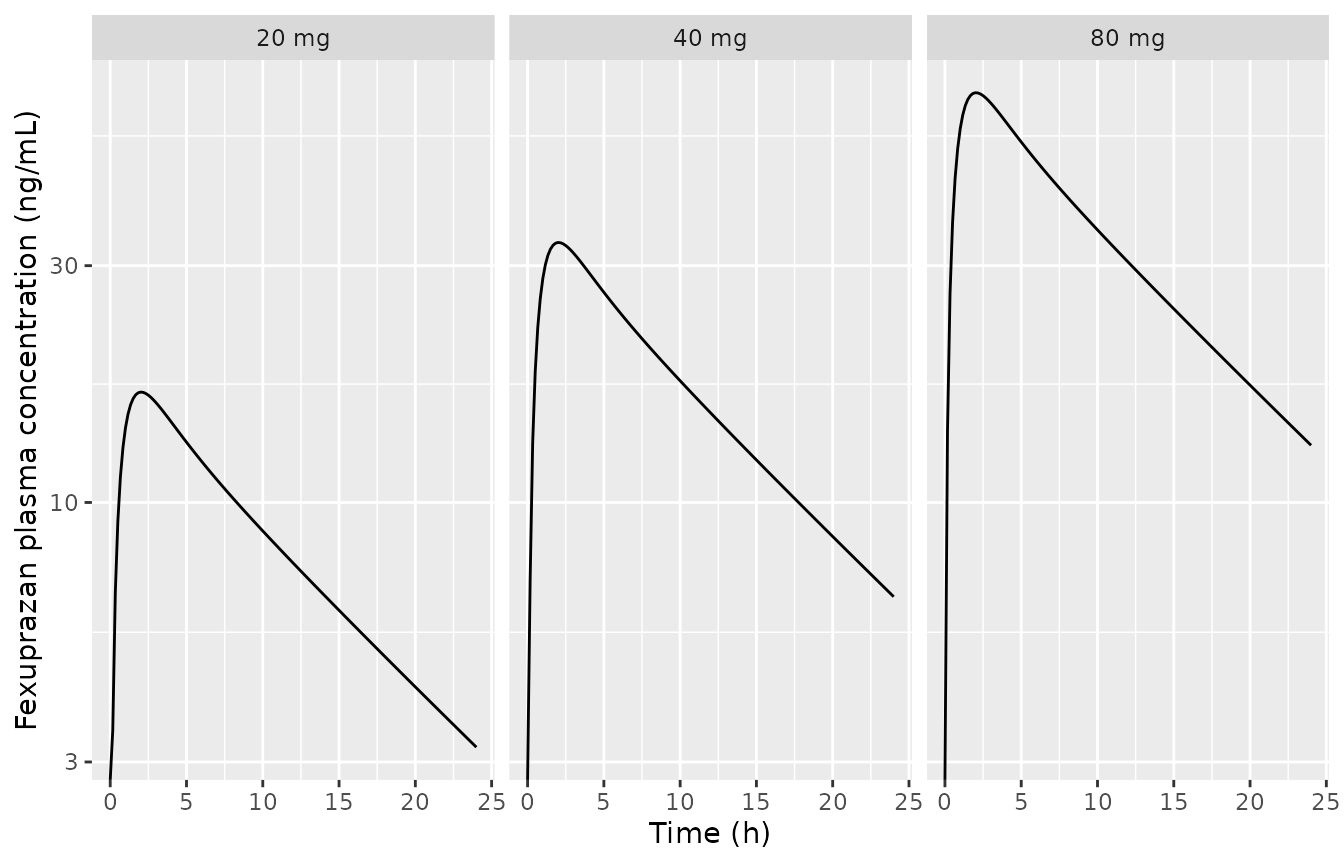
Replicates Figure 2 of Jeong 2021: day-1 plasma concentrations after 20, 40 and 80 mg (typical-value simulation).
sim_mad |>
  ggplot(aes(time / 60, Cc)) +
  geom_line() +
  facet_wrap(~treatment) +
  scale_y_log10() +
  labs(x = "Time (h)", y = "Fexuprazan plasma concentration (ng/mL)")
#> Warning in scale_y_log10(): log-10 transformation introduced infinite values.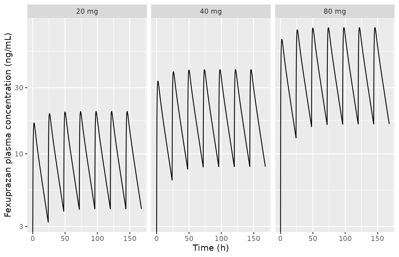
Replicates Figure 3 of Jeong 2021: plasma concentrations over 7 days of once-daily dosing.
Multi-ethnic study (validation set 2)
The Figure 5 caption and x-axis show a single dose on day 1, followed by once-daily dosing on days 5 to 11 (eight doses in total). Sampling ran for 72 h after the first dose (Figure 4) and for 96 h after the eighth dose (Figure 5).
v2_grid <- sort(unique(c(seq(0, 14 * 1440, by = 10), 10 * 1440 + c(0.5, 1, 2, 5))))
v2 <- lapply(c(40, 80), function(d) {
  ev <- rxode2::et(amt = d, cmt = "depot", time = 0) |>
    rxode2::et(amt = d, cmt = "depot", time = 4 * 1440, ii = 1440, addl = 6) |>
    rxode2::et(v2_grid, cmt = "venous") |>
    as.data.frame()
  ev$id <- d
  ev
}) |>
  bind_rows()
sim_v2 <- rxode2::rxSolve(mod_typ, v2, returnType = "data.frame") |>
  as.data.frame() |>
  mutate(treatment = paste(id, "mg"))
#> Warning: multi-subject simulation without without 'omega'
sim_v2 |>
  ggplot(aes(time / 60, Cc)) +
  geom_line() +
  facet_wrap(~treatment) +
  scale_y_log10(limits = c(0.01, NA)) +
  labs(x = "Time (h)", y = "Fexuprazan plasma concentration (ng/mL)")
#> Warning in scale_y_log10(limits = c(0.01, NA)): log-10 transformation
#> introduced infinite values.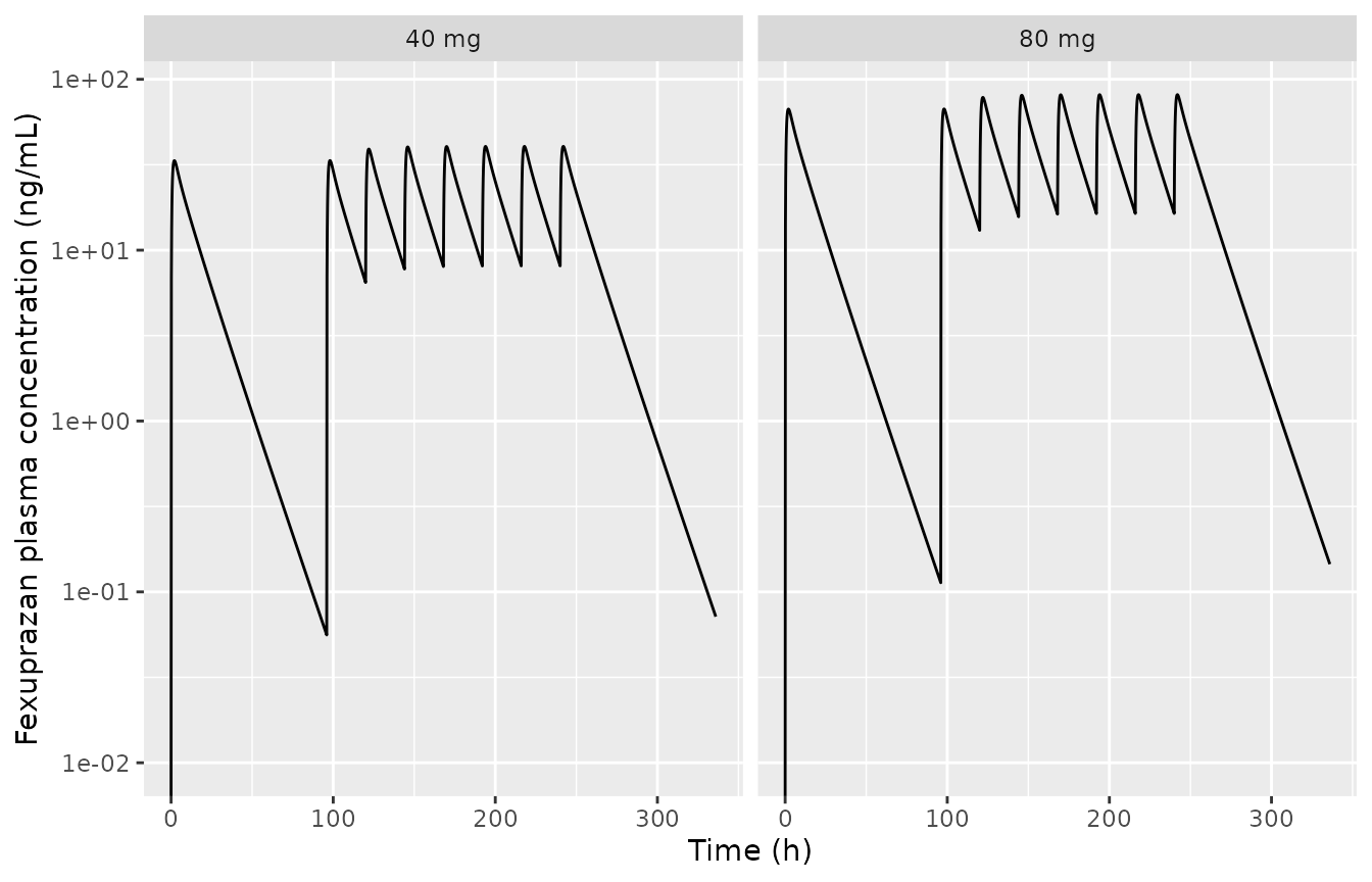
Replicates Figures 4 and 5 of Jeong 2021: first dose (day 1) and once-daily dosing on days 5-11 of 40 and 80 mg.
PKNCA validation
Table 4 reports AUClast and Cmax, both observed and as predicted by the authors’ Berkeley Madonna implementation. The printed AUC unit is “ng min/L”, but the magnitudes only match ng min/mL (for example, 16.6 ng/mL Cmax with a ~9 h half-life). The model-predicted columns are the direct test of this implementation. The observed means are listed alongside for context.
nca_one <- function(sim, intervals) {
  conc <- sim |>
    filter(!is.na(Cc)) |>
    select(id, treatment, time, Cc)
  doses <- sim |>
    distinct(id, treatment) |>
    tidyr::crossing(time = sort(unique(c(0, intervals$start)))) |>
    mutate(amt = id)
  conc_obj <- PKNCA::PKNCAconc(conc, Cc ~ time | treatment + id)
  dose_obj <- PKNCA::PKNCAdose(doses, amt ~ time | treatment + id)
  res <- PKNCA::pk.nca(PKNCA::PKNCAdata(conc_obj, dose_obj, intervals = intervals))
  as.data.frame(res$result)
}
int_mad <- data.frame(
  start = c(0, 6 * 1440), end = c(1440, 7 * 1440),
  cmax = TRUE, auclast = TRUE
)
int_v2 <- data.frame(
  start = c(0, 10 * 1440), end = c(3 * 1440, 14 * 1440),
  cmax = TRUE, auclast = TRUE
)
nca_mad <- nca_one(sim_mad, int_mad) |>
  mutate(set = ifelse(start == 0, "MAD day 1 (training)", "MAD day 7"))
nca_v2 <- nca_one(sim_v2, int_v2) |>
  mutate(set = ifelse(start == 0, "Set 2 first dose", "Set 2 eighth dose"))
nca_all <- bind_rows(nca_mad, nca_v2) |>
  mutate(group = paste(set, treatment, sep = ", ")) |>
  select(group, PPTESTCD, PPORRES)
table4 <- tibble::tribble(
  ~group, ~auclast, ~cmax, ~auc_obs, ~cmax_obs,
  "MAD day 1 (training), 20 mg", 11900, 16.6, 9020, 16.3,
  "MAD day 1 (training), 40 mg", 23900, 33.2, 23700, 40.4,
  "MAD day 1 (training), 80 mg", 48000, 66.6, 62400, 99.1,
  "MAD day 7, 20 mg", 14900, 20.2, 16300, 20.8,
  "MAD day 7, 40 mg", 30000, 40.4, 28300, 43.2,
  "MAD day 7, 80 mg", 60400, 81.2, 68700, 94.4,
  "Set 2 first dose, 40 mg", 29800, 33.2, 21000, 28.8,
  "Set 2 first dose, 80 mg", 60000, 66.6, 66300, 86.4,
  "Set 2 eighth dose, 40 mg", 37500, 40.4, 28300, 35.5,
  "Set 2 eighth dose, 80 mg", 75700, 81.2, 61800, 78.9
)
cmp <- nlmixr2lib::ncaComparisonTable(
  simulated = nca_all,
  reference = table4 |> select(group, auclast, cmax),
  by = "group",
  units = c(cmax = "ng/mL", auclast = "ng*min/mL")
)
obs_long <- bind_rows(
  table4 |> transmute(group, PPTESTCD = "auclast", Observed = auc_obs),
  table4 |> transmute(group, PPTESTCD = "cmax", Observed = cmax_obs)
)
cmp |>
  dplyr::rename("Group" = group, "Paper PBPK prediction" = Reference, "This model" = Simulated) |>
knitr::kable(caption = "Simulated NCA vs. the paper's PBPK predictions (Table 4).")| NCA parameter | Group | Paper PBPK prediction | This model | % diff |
|---|---|---|---|---|
| Cmax (ng/mL) | MAD day 1 (training), 20 mg | 16.6 | 16.7 | +0.5% |
| Cmax (ng/mL) | MAD day 1 (training), 40 mg | 33.2 | 33.4 | +0.6% |
| Cmax (ng/mL) | MAD day 1 (training), 80 mg | 66.6 | 66.9 | +0.5% |
| Cmax (ng/mL) | MAD day 7, 20 mg | 20.2 | 20.2 | -0.0% |
| Cmax (ng/mL) | MAD day 7, 40 mg | 40.4 | 40.5 | +0.2% |
| Cmax (ng/mL) | MAD day 7, 80 mg | 81.2 | 81.3 | +0.1% |
| Cmax (ng/mL) | Set 2 first dose, 40 mg | 33.2 | 33.4 | +0.6% |
| Cmax (ng/mL) | Set 2 first dose, 80 mg | 66.6 | 66.9 | +0.5% |
| Cmax (ng/mL) | Set 2 eighth dose, 40 mg | 40.4 | 40.5 | +0.2% |
| Cmax (ng/mL) | Set 2 eighth dose, 80 mg | 81.2 | 81.3 | +0.1% |
| AUClast (ng*min/mL) | MAD day 1 (training), 20 mg | 11900 | 12000 | +1.1% |
| AUClast (ng*min/mL) | MAD day 1 (training), 40 mg | 23900 | 24100 | +1.0% |
| AUClast (ng*min/mL) | MAD day 1 (training), 80 mg | 48000 | 48500 | +1.1% |
| AUClast (ng*min/mL) | MAD day 7, 20 mg | 14900 | 14900 | +0.0% |
| AUClast (ng*min/mL) | MAD day 7, 40 mg | 30000 | 29900 | -0.2% |
| AUClast (ng*min/mL) | MAD day 7, 80 mg | 60400 | 60400 | -0.0% |
| AUClast (ng*min/mL) | Set 2 first dose, 40 mg | 29800 | 29600 | -0.6% |
| AUClast (ng*min/mL) | Set 2 first dose, 80 mg | 60000 | 59600 | -0.6% |
| AUClast (ng*min/mL) | Set 2 eighth dose, 40 mg | 37500 | 37100 | -1.0% |
| AUClast (ng*min/mL) | Set 2 eighth dose, 80 mg | 75700 | 74900 | -1.0% |
knitr::kable(
  obs_long |> dplyr::rename("Group" = group, "PKNCA code" = PPTESTCD, "Observed mean (Table 4)" = Observed),
  caption = "Observed mean AUClast (ng min/mL) and Cmax (ng/mL) from Table 4, for context."
)| Group | PKNCA code | Observed mean (Table 4) |
|---|---|---|
| MAD day 1 (training), 20 mg | auclast | 9020.0 |
| MAD day 1 (training), 40 mg | auclast | 23700.0 |
| MAD day 1 (training), 80 mg | auclast | 62400.0 |
| MAD day 7, 20 mg | auclast | 16300.0 |
| MAD day 7, 40 mg | auclast | 28300.0 |
| MAD day 7, 80 mg | auclast | 68700.0 |
| Set 2 first dose, 40 mg | auclast | 21000.0 |
| Set 2 first dose, 80 mg | auclast | 66300.0 |
| Set 2 eighth dose, 40 mg | auclast | 28300.0 |
| Set 2 eighth dose, 80 mg | auclast | 61800.0 |
| MAD day 1 (training), 20 mg | cmax | 16.3 |
| MAD day 1 (training), 40 mg | cmax | 40.4 |
| MAD day 1 (training), 80 mg | cmax | 99.1 |
| MAD day 7, 20 mg | cmax | 20.8 |
| MAD day 7, 40 mg | cmax | 43.2 |
| MAD day 7, 80 mg | cmax | 94.4 |
| Set 2 first dose, 40 mg | cmax | 28.8 |
| Set 2 first dose, 80 mg | cmax | 86.4 |
| Set 2 eighth dose, 40 mg | cmax | 35.5 |
| Set 2 eighth dose, 80 mg | cmax | 78.9 |
chk <- nca_all |>
  inner_join(
    bind_rows(
      table4 |> transmute(group, PPTESTCD = "auclast", ref = auclast),
      table4 |> transmute(group, PPTESTCD = "cmax", ref = cmax)
    ),
    by = c("group", "PPTESTCD")
  ) |>
  mutate(pct_diff = 100 * (PPORRES - ref) / ref)
# Deterministic typical-value solves compared with the authors' own
# deterministic predictions: no random draw is involved, so a tight bound on
# every row is appropriate. The residual (at most a few percent) reflects the
# authors' unreported sampling grid for AUClast and their Runge-Kutta step.
stopifnot(nrow(chk) == 20, all(abs(chk$pct_diff) < 5))
All twenty predicted AUClast and Cmax values agree with the paper’s Table 4 predictions to within 5%. Most agree to within about 1%. The largest differences are in the eighth-dose AUCs of set 2, where the exact post-dose sampling window is not printed.
Assumptions and deviations
- Plasma output. The ODEs are written in blood concentrations (Equations 9-13). The paper does not say which pool it reads plasma concentrations from. The model reports venous blood divided by the blood-to-plasma ratio R. Reading arterial blood instead changes day-1 Cmax and AUC by less than 0.5%, and both readings reproduce Table 4.
- Molecular weight. The paper does not print the molecular weight. The model uses 410.4 g/mol for the formula C19H17F3N2O3S. That structure is the M11 N-hydroxylamine named in Section 2.4 without its N-hydroxy oxygen. The value is used only to convert the unbound liver concentration to uM for the Km terms. It does not affect the linear-limit checks above.
-
Residual flow. Equation 11 has a residual flow
QREreturning arterial blood straight to venous blood, but no value is printed. It is taken as the cardiac output minus the flows of the six tissues that drain into venous blood, which closes the venous mass balance. -
Fixed vs. estimated.
FaandCLu,addare the paper’s optimized (fitted) values and are left unfixed. Every physiological, in-vitro or predicted input (includingKa, which came from the Caco-2 correlation) isfixed(). -
No variability. The paper reports the
between-subject SD of the per-subject
FaandCLu,addfits (Results 3.1) but no population variance model and no residual error. The proportional residual error isfixed(0). No between-subject variability is added. - Table 4 AUC unit. The unit is printed as ng min/L but read as ng min/mL, as explained under PKNCA validation.
- Validation set 2 schedule. The dosing (day 1, then days 5-11) and the NCA windows (72 h after the first dose, 96 h after the eighth) were read from the Figure 4 and 5 captions and time axes. The text does not state them.
- Time unit. The model runs in minutes, the paper’s own unit for flows and rate constants.