Isavuconazole + echinocandins against Candida auris in vitro (Caballero 2023)
Source:vignettes/articles/Caballero_2023_isavuconazole_echinocandins.Rmd
Caballero_2023_isavuconazole_echinocandins.RmdModel and source
- Citation: Caballero U, Eraso E, Quindos G, Vozmediano V, Schmidt S, Jauregizar N. PK/PD modeling and simulation of the in vitro activity of the combinations of isavuconazole with echinocandins against Candida auris. CPT Pharmacometrics Syst Pharmacol. 2023;12(6):770-782.
- Article: https://doi.org/10.1002/psp4.12949 (open access, PMC10272309)
- Supplement: Table S1 (the human population PK models used for the clinical simulations), Figures S1-S2 (simulated PK profiles) and Data S1-S3 (the NONMEM control streams for the three combinations).
Caballero et al. fit one semimechanistic PK/PD model per isavuconazole (ISV) + echinocandin combination to static time-kill data on six C. auris blood isolates. The three fits share the structure and have their own parameter set (Table 1), so the package ships three files:
combos <- tibble::tribble(
  ~combination, ~model, ~echinocandin_state, ~control_stream,
  "ISV + anidulafungin (ANF)", "Caballero_2023_isavuconazole_anidulafungin", "canf", "Data S1",
  "ISV + caspofungin (CSP)", "Caballero_2023_isavuconazole_caspofungin", "ccsp", "Data S2",
  "ISV + micafungin (MCF)", "Caballero_2023_isavuconazole_micafungin", "cmcf", "Data S3"
)
knitr::kable(combos)| combination | model | echinocandin_state | control_stream |
|---|---|---|---|
| ISV + anidulafungin (ANF) | Caballero_2023_isavuconazole_anidulafungin | canf | Data S1 |
| ISV + caspofungin (CSP) | Caballero_2023_isavuconazole_caspofungin | ccsp | Data S2 |
| ISV + micafungin (MCF) | Caballero_2023_isavuconazole_micafungin | cmcf | Data S3 |
mods <- lapply(setNames(combos$model, c("anf", "csp", "mcf")), function(nm) rxode2::rxode2(readModelDb(nm)))Model structure
The state log_cfu is the log10 viable count N itself
(the paper’s Nmax is in log CFU/mL and the control streams compare the
prediction A(1) with the log CFU/mL observations
directly):
dN/dt = [kgrow (1 - N / Nmax) (1 - exp(-klag t)) - E] N
The factor (1 - exp(-klag t)) (the paper’s alpha) delays growth at the start of the experiment. Each drug kills through a sigmoid Emax term, E_d = Emax_d C_d^h_d / (EC50_d^h_d + C_d^h_d), and the two kill rates combine through the empirical interaction function of Mohamed et al. 2016 (Equation 3):
E = E_ISV (1 + E_CANDIN / (E_ISV + E_CANDIN))^Int + E_CANDIN (1 + E_ISV / (E_ISV + E_CANDIN))^Int
Each bracket carries the other drug’s effect, so in monotherapy E
reduces to the single drug’s kill rate, and inter > 0
means synergy. The drug concentrations are bath states
(cisv and canf / ccsp /
cmcf, mg/L) with a zero derivative; set them with a dose at
time 0 whose amt is the concentration in mg/L.
Population
This is an in vitro study with no human or animal subjects. The data came from a previously published static time-kill study (Caballero 2021, Antibiotics 10:355) on six C. auris blood isolates (CJ94, CJ97, CJ98, CJ99, CJ100 and CJ102) from an outbreak at the Hospital Universitario y Politecnico La Fe, Valencia, Spain. All six share one MIC per drug (isavuconazole 0.06, anidulafungin 0.125, caspofungin 0.25 and micafungin 0.125 mg/L) and so were classified as wild type. Wells held 200 uL of RPMI medium at 37 C for 48 h, with a starting inoculum of 1-5 x 10^5 CFU/mL. Isavuconazole was tested at 0.125, 0.25, 2 and 4 mg/L and each echinocandin at 0.5-4 mg/L, alone and in combination, alongside a drug-free growth control. Viable counts were taken at 0, 2, 4, 6, 8, 24 and 48 h in independent duplicate experiments (limit of detection 5 CFU/mL).
The models were fit in NONMEM 7.4.3 (FOCE with interaction, ADVAN13) with an additive residual error on log CFU/mL. Neither between-isolate nor between-occasion variability improved the fit, so the final models have none (every OMEGA in Data S1-S3 is fixed to zero).
Source trace
| Quantity | ISV + ANF | ISV + CSP | ISV + MCF | Source |
|---|---|---|---|---|
ODE for N (log_cfu) |
Equations 1-2; Data S1-S3 $DES
|
|||
| Combined effect | Equation 3; Data S1-S3 kanf/kcsp +
kisv
|
|||
lkgrow (kgrowth, 1/h) |
0.158 (fixed) | 0.140 (fixed) | 0.145 (fixed) | Table 1 |
lklag (alpha, 1/h) |
0.162 | 0.161 | 0.158 | Table 1 |
log10cfumax (Nmax, log CFU/mL) |
8 (fixed) | 8 (fixed) | 8 (fixed) | Table 1 |
log10cfu0 (log CFU/mL) |
5.35 (fixed) | 5.35 (fixed) | 5.35 (fixed) | Methods (1-5 x 10^5 CFU/mL); see Assumptions |
lemax_isv (1/h) |
0.0198 | 0.0168 | 0.0176 | Table 1 |
lec50_isv (mg/L) |
0.0683 | 0.0554 | 0.0511 | Table 1 |
hill_isv |
1.58 | 1.16 | 1.12 | Table 1 |
lemax_<candin> (1/h) |
0.0272 | 0.0157 | 0.025 | Table 1 |
lec50_<candin> (mg/L) |
0.176 | 0.452 | 0.171 | Table 1 |
hill_<candin> |
1 (fixed) | 1.37 | 1 (fixed) | Table 1 |
inter (Int) |
0.55 | 1.14 | 0.41 | Table 1 |
addSd (log CFU/mL) |
0.30 | 0.28 | 0.27 | Table 1 |
lapply(mods, function(m) round(m$theta, 4))
#> $anf
#>      lkgrow       lklag log10cfumax   log10cfu0   lemax_isv   lec50_isv
#>     -1.8452     -1.8202      8.0000      5.3500     -3.9221     -2.6838
#>    hill_isv   lemax_anf   lec50_anf    hill_anf       inter       addSd
#>      1.5800     -3.6045     -1.7373      1.0000      0.5500      0.3000
#>
#> $csp
#>      lkgrow       lklag log10cfumax   log10cfu0   lemax_isv   lec50_isv
#>     -1.9661     -1.8264      8.0000      5.3500     -4.0864     -2.8932
#>    hill_isv   lemax_csp   lec50_csp    hill_csp       inter       addSd
#>      1.1600     -4.1541     -0.7941      1.3700      1.1400      0.2800
#>
#> $mcf
#>      lkgrow       lklag log10cfumax   log10cfu0   lemax_isv   lec50_isv
#>     -1.9310     -1.8452      8.0000      5.3500     -4.0399     -2.9740
#>    hill_isv   lemax_mcf   lec50_mcf    hill_mcf       inter       addSd
#>      1.1200     -3.6889     -1.7661      1.0000      0.4100      0.2700
In vitro time-kill: Figures 2 and 3
The arms below are the combination panels of Figure 2 and a subset of the monotherapy panels of Figure 3. Each arm is simulated as 100 replicate wells with the model’s additive residual error; the line is the mean and the band the 95% prediction interval, as in the published VPCs.
arms_combo <- tibble::tribble(
  ~candin, ~isv, ~ech,
  "anf", 0, 0, "anf", 0.06, 0.125, "anf", 0.25, 0.5, "anf", 4, 0.5,
  "anf", 0.25, 1, "anf", 2, 2, "anf", 0.125, 4, "anf", 4, 4,
  "csp", 0, 0, "csp", 0.25, 0.5, "csp", 4, 0.5, "csp", 0.25, 1,
  "csp", 2, 2, "csp", 0.125, 4, "csp", 4, 4,
  "mcf", 0, 0, "mcf", 0.06, 0.125, "mcf", 0.25, 0.5, "mcf", 4, 0.5,
  "mcf", 0.25, 1, "mcf", 2, 2, "mcf", 0.125, 4, "mcf", 4, 4
)
obs_times <- c(0, 2, 4, 6, 8, seq(12, 48, by = 4))

simulate_wells <- function(candin, isv, ech, n_wells = 100) {
  ech_state <- paste0("c", candin)
  doses <- data.frame(time = 0, evid = 1, cmt = c("cisv", ech_state), amt = c(isv, ech))
  doses <- doses[doses$amt > 0, ]
  ev <- do.call(rbind, lapply(seq_len(n_wells), function(i) {
    rbind(
      if (nrow(doses) > 0) cbind(id = i, doses),
      data.frame(id = i, time = obs_times, evid = 0, cmt = "log_cfu", amt = 0)
    )
  }))
  ev <- ev[order(ev$id, ev$time, -ev$evid), ]
  sim <- suppressMessages(suppressWarnings(rxSolve(mods[[candin]], ev, returnType = "data.frame")))
  sim |>
    group_by(time) |>
    summarise(
      mean = mean(sim), lo = quantile(sim, 0.025), hi = quantile(sim, 0.975),
      ipred = mean(log_cfu), .groups = "drop"
    ) |>
    mutate(candin = candin, isv = isv, ech = ech)
}

rxode2::rxSetSeed(20230601)
vpc_combo <- bind_rows(Map(simulate_wells, arms_combo$candin, arms_combo$isv, arms_combo$ech)) |>
  mutate(
    panel = ifelse(isv == 0 & ech == 0, "CONTROL",
      paste0(isv, " mg/L ISV + ", ech, " mg/L ", toupper(candin))
    ),
    candin = toupper(candin)
  )
ggplot(vpc_combo, aes(time, mean)) +
  geom_ribbon(aes(ymin = lo, ymax = hi), fill = "skyblue", alpha = 0.6) +
  geom_line() +
  facet_wrap(~ candin + panel, ncol = 4) +
  coord_cartesian(ylim = c(0, 9)) +
  labs(x = "Time (h)", y = "log CFU/mL") +
  theme_bw(base_size = 8)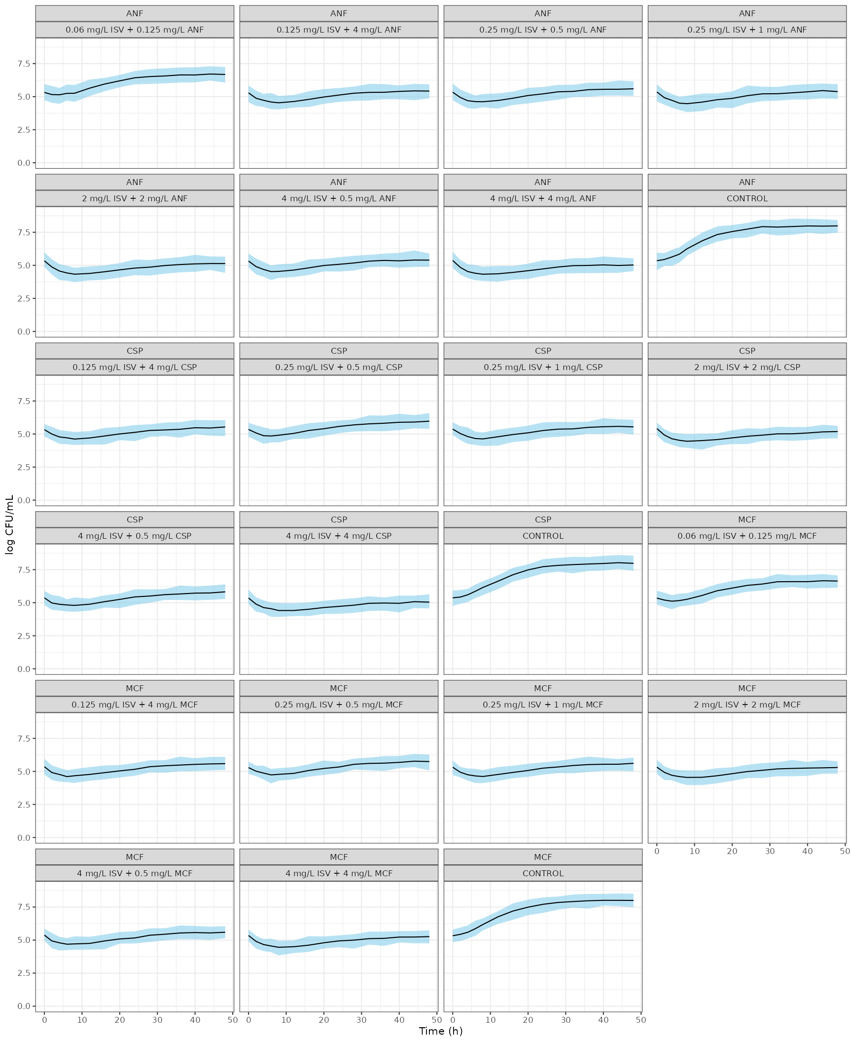
Replicates Figure 2 of Caballero 2023: in vitro time-kill of isavuconazole plus anidulafungin, caspofungin or micafungin (mean and 95% prediction interval of 100 simulated wells).
mono <- bind_rows(
  lapply(c(0.06, 0.25, 1, 4), function(cc) mutate(simulate_wells("anf", cc, 0, 1), drug = "ISV", conc = cc)),
  lapply(c("anf", "csp", "mcf"), function(k) {
    bind_rows(lapply(c(0.25, 1, 4), function(cc) mutate(simulate_wells(k, 0, cc, 1), drug = toupper(k), conc = cc)))
  })
)
ggplot(mono, aes(time, ipred, colour = factor(conc))) +
  geom_line() +
  facet_wrap(~drug, nrow = 1) +
  coord_cartesian(ylim = c(0, 9)) +
  labs(x = "Time (h)", y = "log CFU/mL", colour = "Concentration (mg/L)") +
  theme_bw()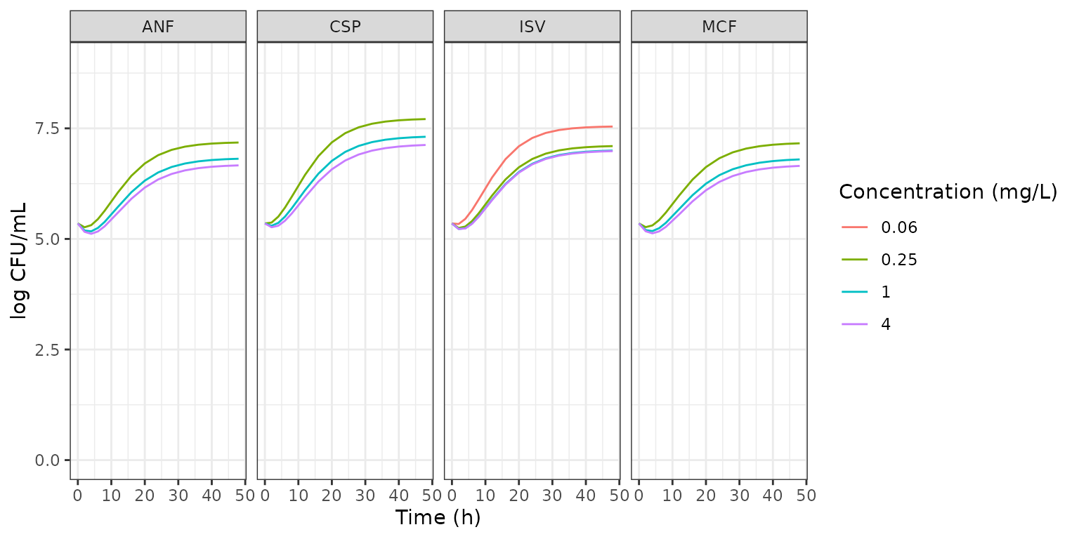
Replicates part of Figure 3 of Caballero 2023: monotherapy arms (typical values) from the ISV + ANF fit (isavuconazole) and from each echinocandin’s own combination fit.
Checks against the published fits
The typical-value curves are compared with values read from Figure 2: the growth controls start near 5.3 log CFU/mL and reach about 8 at 48 h; the 4 mg/L + 4 mg/L combinations fall to a nadir of about 4.4-4.6 log CFU/mL at 6-8 h and recover to about 5 log CFU/mL by 48 h. The comparison is deterministic (typical values), so a tight tolerance is appropriate.
typ <- vpc_combo |>
  filter(panel %in% c("CONTROL", "4 mg/L ISV + 4 mg/L ANF", "4 mg/L ISV + 4 mg/L CSP", "4 mg/L ISV + 4 mg/L MCF")) |>
  group_by(candin, panel) |>
  summarise(
    nadir = min(ipred), t_nadir = time[which.min(ipred)],
    at_48h = ipred[time == 48], .groups = "drop"
  )
knitr::kable(typ, digits = 2)| candin | panel | nadir | t_nadir | at_48h |
|---|---|---|---|---|
| ANF | 4 mg/L ISV + 4 mg/L ANF | 4.32 | 8 | 5.07 |
| ANF | CONTROL | 5.35 | 0 | 7.99 |
| CSP | 4 mg/L ISV + 4 mg/L CSP | 4.41 | 8 | 5.08 |
| CSP | CONTROL | 5.35 | 0 | 7.99 |
| MCF | 4 mg/L ISV + 4 mg/L MCF | 4.47 | 8 | 5.26 |
| MCF | CONTROL | 5.35 | 0 | 7.99 |
ctrl <- filter(typ, panel == "CONTROL")
hi <- filter(typ, panel != "CONTROL")
stopifnot(
  # Logistic growth to Nmax = 8 log CFU/mL by 48 h (Figure 2 controls).
  all(abs(ctrl$at_48h - 8) < 0.1),
  # High-dose combinations: early nadir and partial regrowth (Figure 2).
  all(hi$nadir > 4.2 & hi$nadir < 4.7),
  all(hi$t_nadir >= 4 & hi$t_nadir <= 8),
  all(hi$at_48h > 4.8 & hi$at_48h < 5.4)
)
The interaction function reduces to the single drug’s kill rate when
the other drug is absent, and with inter > 0 a
combination kills faster than the sum of its monotherapy kill rates
(synergy). Both are exact algebraic properties of Equation 3 and are
checked on the packaged parameters:
interaction_rates <- function(m, candin, c_isv, c_ech) {
  th <- m$theta
  e1 <- exp(th[["lemax_isv"]]) * c_isv^th[["hill_isv"]] /
    (exp(th[["lec50_isv"]])^th[["hill_isv"]] + c_isv^th[["hill_isv"]])
  h2 <- th[[paste0("hill_", candin)]]
  e2 <- exp(th[[paste0("lemax_", candin)]]) * c_ech^h2 /
    (exp(th[[paste0("lec50_", candin)]])^h2 + c_ech^h2)
  tot <- e1 + e2
  comb <- e2 * (1 + e1 / tot)^th[["inter"]] + e1 * (1 + e2 / tot)^th[["inter"]]
  c(additive = tot, combined = comb, ratio = comb / tot)
}
syn <- t(sapply(c("anf", "csp", "mcf"), function(k) interaction_rates(mods[[k]], k, 0.25, 0.5)))
knitr::kable(syn, digits = 4, caption = "Kill rates (1/h) at 0.25 mg/L ISV + 0.5 mg/L echinocandin")| additive | combined | ratio | |
|---|---|---|---|
| anf | 0.0377 | 0.0470 | 1.2487 |
| csp | 0.0227 | 0.0351 | 1.5476 |
| mcf | 0.0337 | 0.0397 | 1.1789 |
mono_isv <- sapply(c("anf", "csp", "mcf"), function(k) interaction_rates(mods[[k]], k, 0.25, 0))
mono_ech <- sapply(c("anf", "csp", "mcf"), function(k) interaction_rates(mods[[k]], k, 0, 0.5))
stopifnot(
  all(syn[, "ratio"] > 1),
  # Monotherapy: Equation 3 returns the single drug's own kill rate.
  all(abs(mono_isv["ratio", ] - 1) < 1e-12),
  all(abs(mono_ech["ratio", ] - 1) < 1e-12)
)
Clinical simulations: Figures 4 and 5 and Table 2
Caballero et al. linked the in vitro model to published human population PK models (Table S1) and drove it with unbound concentrations, using protein binding of 98% for isavuconazole, 99% for anidulafungin, 95% for caspofungin and 99.9% for micafungin. The typical PK parameters below come from Table S1; covariate effects (sex and BMI for isavuconazole, SOFA score and BMI for anidulafungin) are not included because Table S1 gives no coefficients. The paper fed the in vitro model typical free concentrations, so these simulations use typical PK.
The PK is added to the packaged model by replacing the zero
derivative of each bath state with a two-compartment disposition written
in unbound-concentration units. Because the system is linear, a dose of
fu * dose / V1 mg/L into the concentration state gives the
unbound central concentration directly.
pk <- tibble::tribble(
  ~drug, ~cl, ~v1, ~v2, ~q, ~fu, ~mic,
  "isv", 4.28, 57.6, 468, 37.4, 0.02, 0.06,
  "anf", 0.89, 12.6, 21.1, 4.4, 0.01, 0.125,
  "csp", 0.55, 8.93, 4.98, 0.71, 0.05, 0.25,
  "mcf", 1.1, 17.6, 3.63, 0.36, 0.001, 0.125
)
knitr::kable(pk, caption = "Typical PK (Table S1; CL and Q in L/h, V in L), unbound fraction and isolate MIC (mg/L)")| drug | cl | v1 | v2 | q | fu | mic |
|---|---|---|---|---|---|---|
| isv | 4.28 | 57.60 | 468.00 | 37.40 | 0.020 | 0.060 |
| anf | 0.89 | 12.60 | 21.10 | 4.40 | 0.010 | 0.125 |
| csp | 0.55 | 8.93 | 4.98 | 0.71 | 0.050 | 0.250 |
| mcf | 1.10 | 17.60 | 3.63 | 0.36 | 0.001 | 0.125 |
link_pk <- function(m, drug) {
  p <- pk[pk$drug == drug, ]
  cs <- paste0("c", drug)
  ps <- paste0("p", drug)
  k10 <- p$cl / p$v1
  k12 <- p$q / p$v1
  k21 <- p$q / p$v2
  e1 <- str2lang(sprintf("d/dt(%s) <- -(%.8g + %.8g) * %s + %.8g * %s", cs, k10, k12, cs, k21, ps))
  e2 <- str2lang(sprintf("d/dt(%s) <- %.8g * %s - %.8g * %s", ps, k12, cs, k21, ps))
  m <- rxode2::model(m, e1)
  rxode2::model(m, e2, append = TRUE)
}
linked <- lapply(c(anf = "anf", csp = "csp", mcf = "mcf"), function(k) {
  suppressMessages(link_pk(link_pk(mods[[k]], "isv"), k))
})
Licensed and alternative regimens (Methods, “PK/PD simulations”), each given as a 1-h intravenous infusion:
q8_then_q24 <- c(seq(0, 40, by = 8), seq(48, 144, by = 24))
daily <- seq(0, 144, by = 24)
regimens <- list(
  isv = list(
    licensed = data.frame(time = q8_then_q24, dose = 200),
    alternative = data.frame(time = q8_then_q24, dose = c(rep(400, 6), rep(200, 5)))
  ),
  anf = list(
    licensed = data.frame(time = daily, dose = c(200, rep(100, 6))),
    alternative = data.frame(time = daily, dose = 200)
  ),
  csp = list(
    licensed = data.frame(time = daily, dose = c(70, rep(50, 6))),
    alternative = data.frame(time = daily, dose = 100)
  ),
  mcf = list(
    licensed = data.frame(time = daily, dose = 100),
    alternative = data.frame(time = daily, dose = 600)
  )
)

dose_rows <- function(drug, regimen) {
  p <- pk[pk$drug == drug, ]
  x <- regimens[[drug]][[regimen]]
  amt <- p$fu * x$dose / p$v1
  data.frame(id = 1, time = x$time, evid = 1, cmt = paste0("c", drug), amt = amt, rate = amt)
}

# EC50 scaled in proportion to the MIC (Equation 4 with d, Emax and h fixed).
mic_params <- function(m, candin, mic_isv, mic_ech) {
  c(
    lec50_isv = m$theta[["lec50_isv"]] + log(mic_isv / pk$mic[pk$drug == "isv"]),
    setNames(
      m$theta[[paste0("lec50_", candin)]] + log(mic_ech / pk$mic[pk$drug == candin]),
      paste0("lec50_", candin)
    )
  )
}

simulate_clinical <- function(candin, reg_isv, reg_ech, mic_isv = NA, mic_ech = NA) {
  ev <- bind_rows(
    dose_rows("isv", reg_isv),
    dose_rows(candin, reg_ech),
    data.frame(id = 1, time = seq(0, 168, by = 2), evid = 0, cmt = "log_cfu", amt = 0, rate = 0)
  )
  m <- rxode2::zeroRe(linked[[candin]])
  prm <- if (is.na(mic_isv)) NULL else mic_params(m, candin, mic_isv, mic_ech)
  out <- suppressMessages(suppressWarnings(rxSolve(m, ev, params = prm, returnType = "data.frame")))
  out[, c("time", "log_cfu", "cisv", paste0("c", candin))]
}
Figure 4: isolate MICs
scen <- tibble::tribble(
  ~scenario, ~reg_isv, ~reg_ech,
  "(a) ISV licensed + candin licensed", "licensed", "licensed",
  "(b) ISV licensed + candin alternative", "licensed", "alternative",
  "(c) ISV alternative + candin licensed", "alternative", "licensed",
  "(d) ISV alternative + candin alternative", "alternative", "alternative"
)
fig4 <- bind_rows(lapply(c("anf", "csp", "mcf"), function(k) {
  bind_rows(lapply(seq_len(nrow(scen)), function(i) {
    simulate_clinical(k, scen$reg_isv[i], scen$reg_ech[i]) |>
      mutate(candin = paste("ISV +", toupper(k)), scenario = scen$scenario[i],
        sd = mods[[k]]$theta[["addSd"]])
  }))
}))
#> Warning: No omega parameters in the model
#> No omega parameters in the model
#> No omega parameters in the model
#> No omega parameters in the model
#> No omega parameters in the model
#> No omega parameters in the model
#> No omega parameters in the model
#> No omega parameters in the model
#> No omega parameters in the model
#> No omega parameters in the model
#> No omega parameters in the model
#> No omega parameters in the model
ggplot(fig4, aes(time / 24, log_cfu)) +
  geom_ribbon(aes(ymin = log_cfu - 1.96 * sd, ymax = log_cfu + 1.96 * sd), fill = "skyblue", alpha = 0.6) +
  geom_line() +
  facet_grid(scenario ~ candin) +
  coord_cartesian(ylim = c(0, 10)) +
  labs(x = "Time (days)", y = "log CFU/mL") +
  theme_bw(base_size = 8)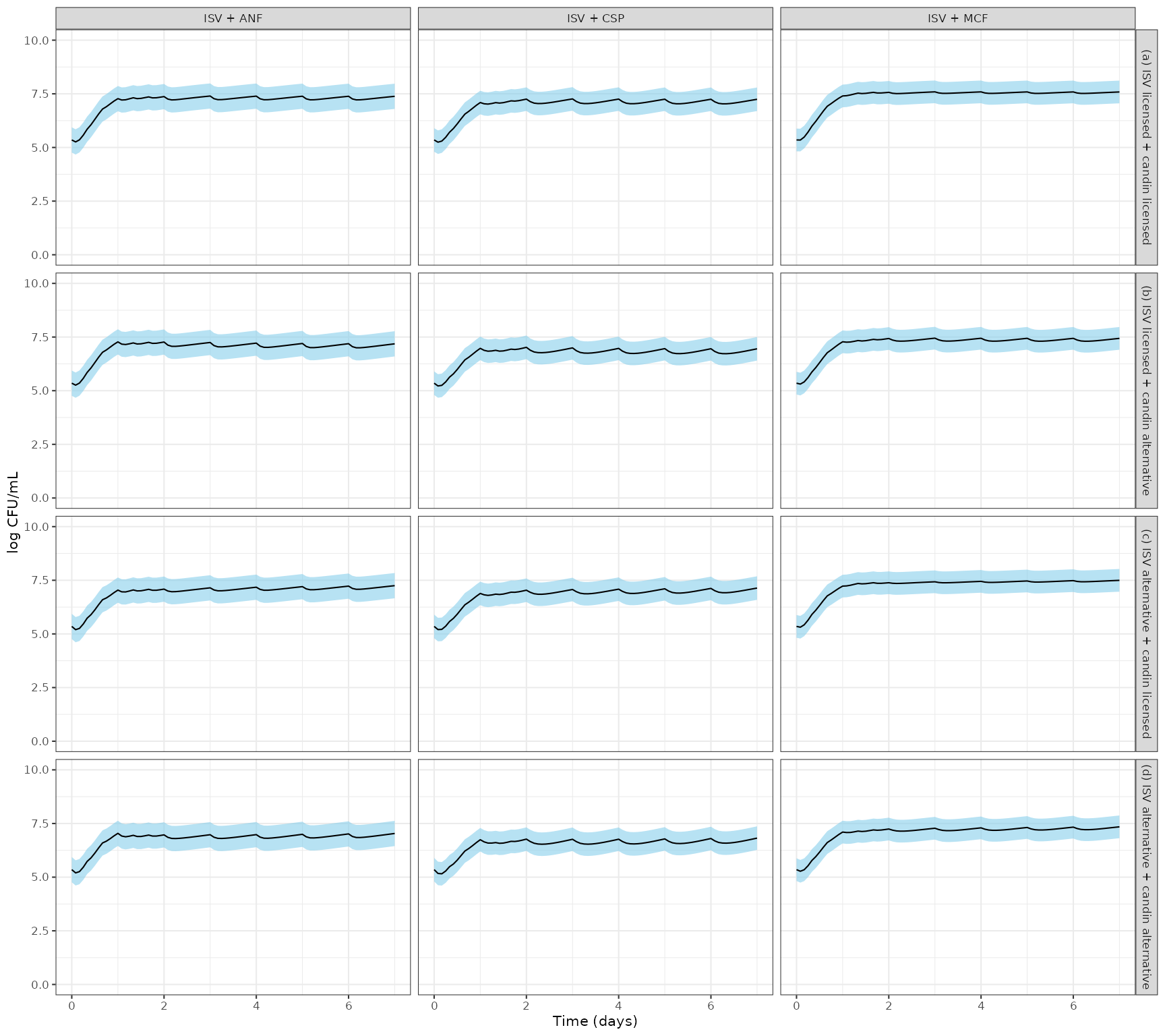
Replicates Figure 4 of Caballero 2023: fungal burden over one week for the four combined dosing scenarios at the MICs of the studied isolates. Line: typical value; band: 95% interval of the additive residual error.
fig4_end <- fig4 |>
  filter(time == 168) |>
  select(candin, scenario, log_cfu)
knitr::kable(fig4_end, digits = 2, caption = "Typical log CFU/mL at day 7")| candin | scenario | log_cfu |
|---|---|---|
| ISV + ANF | (a) ISV licensed + candin licensed | 7.38 |
| ISV + ANF | (b) ISV licensed + candin alternative | 7.18 |
| ISV + ANF | (c) ISV alternative + candin licensed | 7.25 |
| ISV + ANF | (d) ISV alternative + candin alternative | 7.04 |
| ISV + CSP | (a) ISV licensed + candin licensed | 7.24 |
| ISV + CSP | (b) ISV licensed + candin alternative | 6.95 |
| ISV + CSP | (c) ISV alternative + candin licensed | 7.14 |
| ISV + CSP | (d) ISV alternative + candin alternative | 6.82 |
| ISV + MCF | (a) ISV licensed + candin licensed | 7.59 |
| ISV + MCF | (b) ISV licensed + candin alternative | 7.44 |
| ISV + MCF | (c) ISV alternative + candin licensed | 7.50 |
| ISV + MCF | (d) ISV alternative + candin alternative | 7.34 |
Table 2 and Figure 5: lower-MIC scenarios
Caballero et al. derived the EC50 for each MIC scenario from MIC = (d / (Emax - d))^(1/h) x EC50 (Equation 4). The constant d is not reported, but with d, Emax and h unchanged the equation makes EC50 proportional to MIC, so each scenario scales the fitted EC50 by (scenario MIC / isolate MIC).
mic_scen <- tibble::tribble(
  ~scenario, ~mic_isv, ~mic_ech,
  1, 0.015, 0.015, 2, 0.03, 0.015, 3, 0.015, 0.03,
  4, 0.03, 0.03, 5, 0.015, 0.06, 6, 0.03, 0.06
)
grid <- tidyr::expand_grid(
  candin = c("anf", "csp", "mcf"), mic_scen,
  reg_isv = c("licensed", "alternative"), reg_ech = c("licensed", "alternative")
)
grid$day7 <- mapply(function(k, a, b, mi, me) {
  tail(simulate_clinical(k, a, b, mi, me)$log_cfu, 1)
}, grid$candin, grid$reg_isv, grid$reg_ech, grid$mic_isv, grid$mic_ech)
#> Warning: No omega parameters in the model
#> No omega parameters in the model
#> No omega parameters in the model
#> No omega parameters in the model
#> No omega parameters in the model
#> No omega parameters in the model
#> No omega parameters in the model
#> No omega parameters in the model
#> No omega parameters in the model
#> No omega parameters in the model
#> No omega parameters in the model
#> No omega parameters in the model
#> No omega parameters in the model
#> No omega parameters in the model
#> No omega parameters in the model
#> No omega parameters in the model
#> No omega parameters in the model
#> No omega parameters in the model
#> No omega parameters in the model
#> No omega parameters in the model
#> No omega parameters in the model
#> No omega parameters in the model
#> No omega parameters in the model
#> No omega parameters in the model
#> No omega parameters in the model
#> No omega parameters in the model
#> No omega parameters in the model
#> No omega parameters in the model
#> No omega parameters in the model
#> No omega parameters in the model
#> No omega parameters in the model
#> No omega parameters in the model
#> No omega parameters in the model
#> No omega parameters in the model
#> No omega parameters in the model
#> No omega parameters in the model
#> No omega parameters in the model
#> No omega parameters in the model
#> No omega parameters in the model
#> No omega parameters in the model
#> No omega parameters in the model
#> No omega parameters in the model
#> No omega parameters in the model
#> No omega parameters in the model
#> No omega parameters in the model
#> No omega parameters in the model
#> No omega parameters in the model
#> No omega parameters in the model
#> No omega parameters in the model
#> No omega parameters in the model
#> No omega parameters in the model
#> No omega parameters in the model
#> No omega parameters in the model
#> No omega parameters in the model
#> No omega parameters in the model
#> No omega parameters in the model
#> No omega parameters in the model
#> No omega parameters in the model
#> No omega parameters in the model
#> No omega parameters in the model
#> No omega parameters in the model
#> No omega parameters in the model
#> No omega parameters in the model
#> No omega parameters in the model
#> No omega parameters in the model
#> No omega parameters in the model
#> No omega parameters in the model
#> No omega parameters in the model
#> No omega parameters in the model
#> No omega parameters in the model
#> No omega parameters in the model
#> No omega parameters in the model

grid |>
  mutate(regimen = paste0("ISV ", reg_isv, " / candin ", reg_ech)) |>
  select(candin, scenario, mic_isv, mic_ech, regimen, day7) |>
  tidyr::pivot_wider(names_from = regimen, values_from = day7) |>
knitr::kable(digits = 2, caption = "Typical log CFU/mL at day 7 by MIC scenario and regimen")| candin | scenario | mic_isv | mic_ech | ISV licensed / candin licensed | ISV licensed / candin alternative | ISV alternative / candin licensed | ISV alternative / candin alternative |
|---|---|---|---|---|---|---|---|
| anf | 1 | 0.01 | 0.01 | 5.95 | 5.73 | 5.84 | 5.61 |
| anf | 2 | 0.03 | 0.01 | 6.29 | 6.08 | 6.11 | 5.89 |
| anf | 3 | 0.01 | 0.03 | 6.25 | 5.96 | 6.14 | 5.85 |
| anf | 4 | 0.03 | 0.03 | 6.56 | 6.30 | 6.40 | 6.12 |
| anf | 5 | 0.01 | 0.06 | 6.55 | 6.25 | 6.45 | 6.15 |
| anf | 6 | 0.03 | 0.06 | 6.84 | 6.57 | 6.69 | 6.40 |
| csp | 1 | 0.01 | 0.01 | 5.58 | 5.51 | 5.47 | 5.40 |
| csp | 2 | 0.03 | 0.01 | 5.88 | 5.82 | 5.72 | 5.65 |
| csp | 3 | 0.01 | 0.03 | 5.74 | 5.58 | 5.64 | 5.48 |
| csp | 4 | 0.03 | 0.03 | 6.03 | 5.88 | 5.88 | 5.72 |
| csp | 5 | 0.01 | 0.06 | 6.04 | 5.75 | 5.95 | 5.64 |
| csp | 6 | 0.03 | 0.06 | 6.30 | 6.03 | 6.16 | 5.88 |
| mcf | 1 | 0.01 | 0.01 | 7.01 | 6.43 | 6.95 | 6.35 |
| mcf | 2 | 0.03 | 0.01 | 7.19 | 6.62 | 7.10 | 6.52 |
| mcf | 3 | 0.01 | 0.03 | 7.13 | 6.70 | 7.07 | 6.63 |
| mcf | 4 | 0.03 | 0.03 | 7.30 | 6.88 | 7.21 | 6.79 |
| mcf | 5 | 0.01 | 0.06 | 7.20 | 6.92 | 7.13 | 6.85 |
| mcf | 6 | 0.03 | 0.06 | 7.36 | 7.09 | 7.28 | 7.00 |
fig5 <- bind_rows(lapply(seq_len(nrow(mic_scen)), function(i) {
  simulate_clinical("csp", "alternative", "alternative", mic_scen$mic_isv[i], mic_scen$mic_ech[i]) |>
    mutate(scenario = paste("Scenario", mic_scen$scenario[i]))
}))
#> Warning: No omega parameters in the model
#> No omega parameters in the model
#> No omega parameters in the model
#> No omega parameters in the model
#> No omega parameters in the model
#> No omega parameters in the model
ctrl_ev <- data.frame(id = 1, time = seq(0, 168, by = 2), evid = 0, cmt = "log_cfu", amt = 0)
control <- suppressMessages(suppressWarnings(
  rxSolve(rxode2::zeroRe(mods$csp), ctrl_ev, returnType = "data.frame")
))
ggplot(fig5, aes(time / 24, log_cfu)) +
  geom_line(data = control, colour = "grey30") +
  geom_line(colour = "magenta") +
  facet_wrap(~scenario) +
  coord_cartesian(ylim = c(0, 10)) +
  labs(x = "Time (days)", y = "log CFU/mL") +
  theme_bw()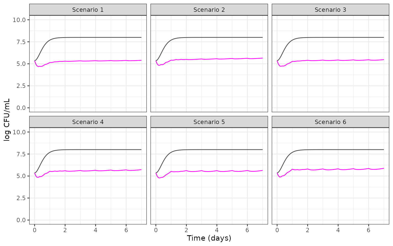
Replicates Figure 5 of Caballero 2023: alternative isavuconazole (400 mg every 8 h for 48 h, then 200 mg daily) plus alternative caspofungin (100 mg daily) for the six MIC scenarios; grey line, growth control.
fig5_end <- fig5 |>
  filter(time == 168)
stopifnot(
  # Figure 5: the treated arm plateaus between about 5.3 (scenario 1) and
  # 5.9 (scenario 6) log CFU/mL, far below the growth control at 8.
  all(fig5_end$log_cfu > 5.2 & fig5_end$log_cfu < 6.1),
  abs(tail(control$log_cfu, 1) - 8) < 0.05,
  # Ranking reported in the Results and Discussion: the micafungin
  # combination is the least active in every MIC scenario and regimen.
  all(
    grid$day7[grid$candin == "mcf"] > grid$day7[grid$candin == "csp"],
    grid$day7[grid$candin == "mcf"] > grid$day7[grid$candin == "anf"]
  )
)
The ranking matches the paper: caspofungin is the most active partner, anidulafungin intermediate and micafungin the least active. The packaged values reproduce Figure 5 closely. Table 2’s exact pass/fail boundaries are not reproduced one-for-one, because the paper does not state the numerical criterion for “fungal growth was inhibited”. Its pass/fail split lies roughly between 6.0 and 6.3 log CFU/mL on the typical day-7 values above.
Assumptions and deviations
-
Starting inoculum. The control streams enter each
well’s starting count through
AMTinto the fungal compartment, so the paper reports no single value.log10cfu0is fixed at 5.35 log CFU/mL, the log10 of the geometric midpoint of the stated 1-5 x 10^5 CFU/mL range; it matches the start of the Figure 2 VPCs (about 5.3). Override it withini()to simulate another inoculum. -
Drug-free control. Equation 3 is 0/0 when both
concentrations are zero. The packaged model sets the kill rate to zero
in that case; the control streams reach the same result by switching the
ODE on a
TYPEdata column (1 = echinocandin alone, 2 = isavuconazole alone, 3 = combination, 4 = control). Because Equation 3 reduces exactly to the single-drug kill rate in monotherapy, one ODE covers all four types. - EC50 of isavuconazole in the ISV + MCF fit. The Results text quotes 0.0584 mg/L, but Table 1 prints 0.0511 mg/L with a bootstrap 95% CI of 0.0476-0.0543, which excludes 0.0584. The table value is used.
-
Residual error. Table 1 reports sigma in log CFU/mL
units, so it is taken as an additive standard deviation
(
addSd). - Clinical simulations. These are reproduced in this article and are not part of the packaged models. The PK models (Wu 2020 isavuconazole, Kapralos 2021 anidulafungin, Martial 2016 caspofungin, Martial 2017 micafungin) are used at the typical values in Table S1, without covariate effects (Table S1 gives no coefficients) and with 1-h infusions (the paper does not state infusion durations). The figure bands show the PD residual error around the typical prediction, which approximately matches the width of the published Figure 4 bands.
- MIC scenarios. Equation 4 was applied with the constant d, Emax and h unchanged, which makes EC50 proportional to MIC (d is not reported).
- No between-isolate or between-occasion variability, as in the published final models.