Doxorubicin cardiotoxicity QSP, rat and human (Sang 2021)
Source:vignettes/articles/Sang_2021_doxorubicin_cardiotoxicity.Rmd
Sang_2021_doxorubicin_cardiotoxicity.RmdModel and source
- Citation: Sang L, Yuan Y, Zhou Y, Zhou Z, Jiang M, Liu X, Hao K, He H (2021). A quantitative systems pharmacology approach to predict the safe-equivalent dose of doxorubicin in patients with cardiovascular comorbidity. CPT Pharmacometrics Syst Pharmacol. 10(12):1512-1524. doi:10.1002/psp4.12719. Structure and constants from the deposited Mlxtran code (Supporting Information, ‘Mlxtran code for rat QSP/PK/PD model’) and Tables S4-S5. Afterload model from Snelder N et al. (2014) Br J Pharmacol 171:5076-5092.
- Article: https://doi.org/10.1002/psp4.12719
Sang et al. (2021) built a quantitative systems pharmacology (QSP) model of doxorubicin-induced cardiac dysfunction in rats and translated it to humans to estimate a “safe-equivalent” cumulative dose for patients with pre-existing cardiovascular disease. The paper contributes two model files:
-
Sang_2021_doxorubicin_rat_qsp– the fitted rat QSP-PK-PD model: a five-compartment doxorubicin PK model (intraperitoneal depot, plasma, heart, two peripheral compartments) feeding a cumulative heart-tissue AUC, which impairs bioenergy production and myocardial compliance inside a cardiovascular turnover system (stroke volume SV, left ventricular end-diastolic volume LVEDV, heart rate HR, total peripheral resistance TPR; MAP = HR x TPR x SV; LVESV = LVEDV - SV; LVEF = SV / LVEDV). -
Sang_2021_doxorubicin_human_qsp– the human translation (Table 1): the dissipation rate constants are allometrically scaled, FB_LVESV is rescaled by the baseline LVESV, and only the bioenergy-production (systolic) arm is retained. The paper obtained human heart exposure from the separately published He 2018 multiscale doxorubicin PBPK model, which is not part of nlmixr2lib, so this file takes the heart-tissue doxorubicin concentration as the time-varying covariateCEFFECT(ug/mL).
The rat structure and every constant come from the Mlxtran code the authors deposited with the Supporting Information; the parameter values match Tables S4 and S5 except where noted under “Assumptions and deviations”.
Population
Rat. The PK model was fitted first to ten literature PK studies (2-6 mg/kg single i.v. or i.p. doses in Wistar-Kyoto, Sprague-Dawley, Donryu and BDIX rats; Table S1) and then fixed. The QSP and PD parameters were estimated jointly (Monolix 2018R1, SAEM) on three literature echocardiography studies in Sprague-Dawley rats (Chang 2015, Kim 2012, Lee 2014; 90 rats, 1.25-3 mg/kg i.p. repeated doses) and an in-house study of 3.75 mg/kg i.p. every 3 days for 4 doses in healthy Wistar-Kyoto (WKY) rats, isoproterenol-hypertrophied WKY rats and spontaneously hypertensive rats (SHR). Body weights were 250-329 g (Table S1).
Human. No human data were fitted. 13,994 virtual adult patients (8599 cardiovascular-healthy, 5395 with enlarged LVEDV and/or hypertension) were generated by Monte Carlo sampling of the Table 1 baselines with 30% variation and simulated for one year of 3-weekly doxorubicin (cumulative 120-900 mg/m^2).
str(readModelDb("Sang_2021_doxorubicin_rat_qsp")()$population)
#> List of 7
#>  $ species      : chr "rat (Sprague-Dawley, Wistar-Kyoto, spontaneously hypertensive)"
#>  $ n_subjects   : num 114
#>  $ n_studies    : num 6
#>  $ weight_range : chr "250-329 g (study means, PD studies; Table S1)"
#>  $ disease_state: chr "Doxorubicin-induced cardiac dysfunction in healthy rats, isoproterenol-induced myocardial hypertrophy (WKY) and"| __truncated__
#>  $ dose_range   : chr "1.25-3.75 mg/kg intraperitoneal, 4-16 doses (PD studies 11-14); PK from 2-6 mg/kg i.v. or i.p. single doses (studies 1-10)"
#>  $ notes        : chr "QSP and PD parameters estimated jointly (Monolix 2018R1 SAEM) on three literature studies (Chang 2015, Kim 2012"| __truncated__
str(readModelDb("Sang_2021_doxorubicin_human_qsp")()$population)
#> List of 6
#>  $ species      : chr "human"
#>  $ n_subjects   : num 13994
#>  $ disease_state: chr "Virtual adult cancer patients treated with doxorubicin, with (n = 5395) or without (n = 8599) cardiovascular co"| __truncated__
#>  $ weight_range : chr "70 kg typical (CV 30%)"
#>  $ dose_range   : chr "Cumulative doxorubicin 120-900 mg/m^2, infused every 3 weeks over 1 year"
#>  $ notes        : chr "Virtual population only; no human data were fitted. Physiological baselines drawn by Monte Carlo with 30% varia"| __truncated__
Source trace
| Equation / parameter | Rat value | Human value | Source location |
|---|---|---|---|
LVEDV turnover (d/dt(edv)) |
– | – | Eq. 1; Mlxtran ddt_LVEDV
|
| LVESV = LVEDV - SV; LVEF = SV/LVEDV | – | – | Eqs. 2-3; Mlxtran |
| HR, TPR, SV turnover | – | – | Eqs. 4-6; Mlxtran ddt_HR, ddt_TPR,
ddt_SV
|
| MAP = HR x TPR x SV | – | – | Eq. 7 |
| FB_MAP = FB_MAP_0 (MAP_base/MAP_0)^-1.98 | MAP_0 = 106.596 | 106.596 | Eq. 8; Mlxtran FB_MAP
|
| E_drug_EP = exp(-AUCh/(AUCh + AUC50_EP^h)) | – | – | Eq. 9; Mlxtran EdrugEP, EEP_SV
|
| MC transit chain and E_MC_LVEDV = 1 - MC_T3 | – | not used | Eqs. 10-12; Mlxtran MCtrans1-3
|
| E_MC_SV = 1 - AUC/(AUC + AUC50_MC) | – | not used | Eq. 13; Mlxtran EMC_SV
|
| Allometric scaling of kout, exponent -0.25 | – | – | Eq. 14 |
| FB_LVESV scaled by baseline LVESV ratio | – | – | Eq. 15 |
lka |
4.532 1/h | – | Mlxtran k; Table S4 ka 4.53 |
lkel |
1.07 1/h | – | Mlxtran ke; Table S4 |
lvc |
442 mL | – | Mlxtran V1; Table S4 |
lv_heart |
60.5 mL | – | Mlxtran V2; Table S4 |
lkin_heart, lkout_heart
|
6.75, 0.605 1/h | – | Mlxtran K12, K21; Table S4 k_in_heart,
k_out_heart |
lk12, lk21
|
6.74, 13.4 1/h | – | Mlxtran K13, K31; Table S4 k12, k21 |
lk13, lk31
|
3.07, 0.0568 1/h | – | Mlxtran K14, K41; Table S4 k13, k31
(0.0586) |
lrbase_hr / HR_BL
|
423 beats/min (fixed) | covariate (70) | Mlxtran HR0; Table S5 / Table 1 |
lkout_hr |
11.58 1/h | 2.83 1/h | Mlxtran; Table 1 |
lkout_tpr |
3.58 1/h | 0.875 1/h | Mlxtran; Table 1 |
lkout_edv |
0.126 1/h | 0.0308 1/h | Mlxtran; Table 1 |
lkout_sv |
0.126 1/h | 0.0308 1/h | Table S5; Table 1 |
lfb0 |
0.0029 1/mmHg | 0.0029 1/mmHg | Mlxtran; Table 1 FB_MAP_0 |
e_bslmap_fb |
-1.98 | -1.98 | Methods (Snelder 2014) |
lfb_lvesv |
1.43 1/mL | 2.532e-3 1/mL | Table S5; Table 1 |
lktr |
0.021 1/h | – | Table S5 kt |
lauc50_ep |
1390 ug*h/mL | 1390 ug*h/mL | Table S5; Table 1 |
lauc50_mc |
1704 ug*h/mL | – | Table S5 |
hill_ep, hill_mc
|
3, 1 | 3, – | Results; Mlxtran |
etalfb_lvesv, etalauc50_ep
|
– | CV 12.4%, 7.06% | Table 1 CV column |
| Residual errors | not reported (fixed 0) | not reported (fixed 0) | Supplementary Methods Eqs. 1-4 |
Rat model
mod_rat <- readModelDb("Sang_2021_doxorubicin_rat_qsp")
rat_ui <- rxode2::rxode2(mod_rat)
rat_par <- setNames(rat_ui$iniDf$est, rat_ui$iniDf$name)
Doxorubicin PK (Figure S2)
Figure S2 shows plasma and heart concentrations after a 5 mg/kg dose. The deposited code works in per-animal amounts, so a 5 mg/kg dose to a 250 g rat is 1250 ug; the resulting heart peak of about 11 ug/mL and plasma concentration of about 20 ng/mL at 24 h match the Figure S2 axes (in ng/mL).
dose_ug <- 5 * 0.250 * 1000
t_pk <- sort(unique(c(0, 10^seq(-3, log10(2000), length.out = 300), 24, 48, 72)))
pk_events <- dplyr::bind_rows(
  data.frame(id = 1L, time = 0, evid = 1L, amt = dose_ug, cmt = "central", treatment = "5 mg/kg i.v."),
  data.frame(id = 1L, time = t_pk, evid = 0L, amt = 0, cmt = NA_character_, treatment = "5 mg/kg i.v."),
  data.frame(id = 2L, time = 0, evid = 1L, amt = dose_ug, cmt = "depot", treatment = "5 mg/kg i.p."),
  data.frame(id = 2L, time = t_pk, evid = 0L, amt = 0, cmt = NA_character_, treatment = "5 mg/kg i.p.")
) |>
  dplyr::mutate(dvid = ifelse(evid == 0L, 1L, NA_integer_), LVEDV_BL = 0.385, LVESV_BL = 0.085, MAP_BL = 106.596, STRAIN_SD = 1)

pk_sim <- rxode2::rxSolve(mod_rat, pk_events, keep = "treatment", returnType = "data.frame",
                          atol = 1e-10, rtol = 1e-10, maxsteps = 1e6)
#> Warning: multi-subject simulation without without 'omega'

# The time-zero row (concentration 0) is left out of this log-scale plot only;
# the PKNCA input below keeps it.
pk_long <- pk_sim[pk_sim$time > 0, ] |>
  dplyr::select(treatment, time, Plasma = Cc, Heart = Cheart) |>
  tidyr::pivot_longer(c(Plasma, Heart), names_to = "matrix", values_to = "conc")

ggplot(pk_long, aes(time, conc * 1000, colour = treatment)) +
  geom_line() +
  facet_wrap(~matrix) +
  scale_y_log10() +
  coord_cartesian(xlim = c(0, 72)) +
  labs(x = "Time (h)", y = "Doxorubicin (ng/mL)", colour = NULL,
       caption = "Replicates Figure S2 of Sang 2021 (predicted median).")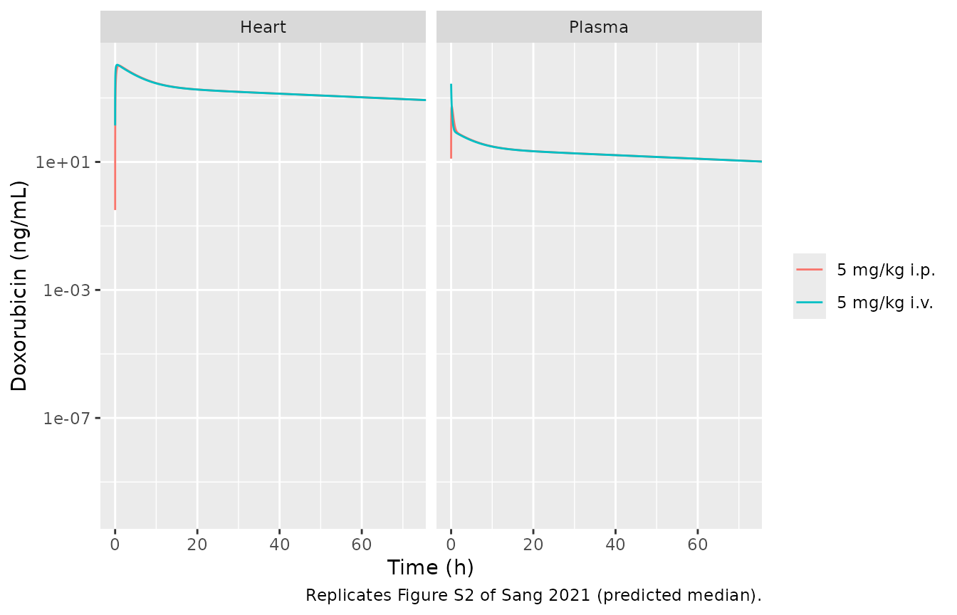
pk_iv <- pk_sim[pk_sim$treatment == "5 mg/kg i.v.", ]
heart_peak <- max(pk_iv$Cheart)
plasma_24 <- pk_iv$Cc[pk_iv$time == 24] * 1000
knitr::kable(data.frame(
  Quantity = c("Heart Cmax (ug/mL)", "Plasma at 24 h (ng/mL)"),
  Simulated = signif(c(heart_peak, plasma_24), 3),
  "Figure S2" = c("about 10 (1e4 ng/mL axis)", "about 15-20"),
  check.names = FALSE
))| Quantity | Simulated | Figure S2 |
|---|---|---|
| Heart Cmax (ug/mL) | 10.8 | about 10 (1e4 ng/mL axis) |
| Plasma at 24 h (ng/mL) | 20.2 | about 15-20 |
stopifnot(heart_peak > 5, heart_peak < 20, plasma_24 > 10, plasma_24 < 40)NCA (PKNCA)
The paper reports no NCA table for the rat PK, so the NCA here checks the implementation against its own mass balance: plasma AUC(0-inf) must equal Dose / (kel * V1) for both routes (i.p. absorption is complete), and the heart AUC follows from the heart-to-plasma exchange.
nca_conc <- pk_sim |>
  dplyr::filter(!is.na(Cc)) |>
  dplyr::select(id, treatment, time, Cc)
nca_dose <- pk_events |>
  dplyr::filter(evid == 1L) |>
  dplyr::select(id, treatment, time, amt)
conc_obj <- PKNCA::PKNCAconc(nca_conc, Cc ~ time | treatment + id)
dose_obj <- PKNCA::PKNCAdose(nca_dose, amt ~ time | treatment + id)
intervals <- data.frame(start = 0, end = Inf, cmax = TRUE, tmax = TRUE,
                        aucinf.obs = TRUE, half.life = TRUE)
nca_res <- PKNCA::pk.nca(PKNCA::PKNCAdata(conc_obj, dose_obj, intervals = intervals))
nca_tab <- as.data.frame(nca_res$result) |>
  dplyr::filter(PPTESTCD %in% c("cmax", "tmax", "aucinf.obs", "half.life")) |>
  dplyr::select(treatment, PPTESTCD, PPORRES) |>
  tidyr::pivot_wider(names_from = PPTESTCD, values_from = PPORRES)
nca_tab |>
  dplyr::rename("Route" = treatment, "Cmax (ug/mL)" = cmax, "Tmax (h)" = tmax,
                "AUC0-inf (ug*h/mL)" = aucinf.obs, "t1/2 (h)" = half.life) |>
knitr::kable(digits = 4)| Route | Cmax (ug/mL) | Tmax (h) | t1/2 (h) | AUC0-inf (ug*h/mL) |
|---|---|---|---|---|
| 5 mg/kg i.p. | 0.5389 | 0.1481 | 53.5383 | 2.6432 |
| 5 mg/kg i.v. | 2.8281 | 0.0000 | 53.5295 | 2.6432 |
auc_expected <- dose_ug / (exp(rat_par[["lkel"]]) * exp(rat_par[["lvc"]]))
auc_pct <- 100 * (nca_tab$aucinf.obs / auc_expected - 1)
heart_expected <- auc_expected * exp(rat_par[["lvc"]]) * exp(rat_par[["lkin_heart"]]) /
  exp(rat_par[["lkout_heart"]]) / exp(rat_par[["lv_heart"]])
heart_pct <- 100 * (tail(pk_iv$auc_heart, 1) / heart_expected - 1)
c(expected_plasma_auc = auc_expected, pct_diff = auc_pct,
  expected_heart_auc = heart_expected, heart_state_pct_diff = heart_pct)
#>  expected_plasma_auc            pct_diff1            pct_diff2
#>         2.643041e+00         4.465389e-03         4.964172e-03
#>   expected_heart_auc heart_state_pct_diff
#>         2.154365e+02        -4.955591e-10
stopifnot(all(abs(auc_pct) < 2), abs(heart_pct) < 1)
Pre-dose steady state
With no dose, every turnover state must stay at its baseline: the production rates are derived from the pre-dose steady state.
ss_events <- data.frame(id = 1L, time = c(0, 24, 240, 2400), evid = 0L, amt = 0, dvid = 1L,
                        LVEDV_BL = 0.385, LVESV_BL = 0.085, MAP_BL = 106.596, STRAIN_SD = 0)
ss <- rxode2::rxSolve(mod_rat, ss_events, returnType = "data.frame")
ss[, c("time", "LVEF", "LVEDV", "LVESV", "MAP", "hr", "tpr")]
#>   time     LVEF LVEDV LVESV     MAP  hr  tpr
#> 1    0 77.92208 0.385 0.085 106.596 423 0.84
#> 2   24 77.92208 0.385 0.085 106.596 423 0.84
#> 3  240 77.92208 0.385 0.085 106.596 423 0.84
#> 4 2400 77.92208 0.385 0.085 106.596 423 0.84
stopifnot(
  max(abs(ss$LVEDV / 0.385 - 1)) < 1e-6,
  max(abs(ss$LVESV / 0.085 - 1)) < 1e-6,
  max(abs(ss$MAP / 106.596 - 1)) < 1e-6
)
Figure 2 and Table S2
The panels of Figure 2 are typical-value predictions using each study’s own baselines. Doses are per-animal (mg/kg x study body weight from Table S1). Baselines for studies 11-13 are read from the starting point of the Figure 2 curves; for the in-house groups 14A-C they are the Table S2 day-0 means. Dosing intervals for the literature studies are read from the Figure 2 arrows; the in-house schedule is every 3 days for 4 doses (Supplementary Methods).
studies <- data.frame(
  study = c("11", "12", "13", "14A", "14B", "14C"),
  STRAIN_SD = c(1, 1, 1, 0, 0, 0),
  dose_ug = c(3 * 275, 1.25 * 329.3, 2.5 * 250, 3.75 * 250, 3.75 * 250, 3.75 * 250),
  n_dose = c(6, 16, 6, 4, 4, 4),
  ii = c(168, 55, 46, 72, 72, 72),
  lvef_bl = c(78, 80, 85, (1 - 75.6 / 264.2) * 100,
              (1 - 96.8 / 292.3) * 100, (1 - 107.3 / 300.3) * 100),
  lvedv_bl = c(0.37, 0.39, 0.34, 0.2642, 0.2923, 0.3003),
  map_bl = c(106.596, 106.596, 106.596, 112.7, 120.3, 156.7),
  tend = c(1344, 1344, 1008, 384, 384, 384)
)
studies$lvesv_bl <- studies$lvedv_bl * (1 - studies$lvef_bl / 100)

make_study <- function(i) {
  s <- studies[i, ]
  obs <- sort(unique(c(seq(0, s$tend, by = 4), 96, 192, 360)))
  dplyr::bind_rows(
    data.frame(time = (seq_len(s$n_dose) - 1) * s$ii, evid = 1L, amt = s$dose_ug, cmt = "depot", dvid = NA_integer_),
    data.frame(time = obs, evid = 0L, amt = 0, cmt = NA_character_, dvid = 1L)
  ) |>
    dplyr::mutate(id = i, study = s$study, STRAIN_SD = s$STRAIN_SD,
                  LVEDV_BL = s$lvedv_bl, LVESV_BL = s$lvesv_bl, MAP_BL = s$map_bl)
}
rat_events <- dplyr::bind_rows(lapply(seq_len(nrow(studies)), make_study)) |>
  dplyr::arrange(id, time, dplyr::desc(evid))
rat_sim <- rxode2::rxSolve(mod_rat, rat_events, keep = "study", returnType = "data.frame",
                           maxsteps = 1e6)

rat_sim |>
  dplyr::select(study, time, "LVEF (%)" = LVEF, "LVEDV (mL)" = LVEDV) |>
  tidyr::pivot_longer(-c(study, time)) |>
  ggplot(aes(time, value)) +
  geom_line(colour = "red") +
  facet_grid(name ~ study, scales = "free") +
  labs(x = "Time since first dose (h)", y = NULL,
       caption = "Replicates Figure 2 of Sang 2021 (a: studies 11-13; b: study 14A-C).")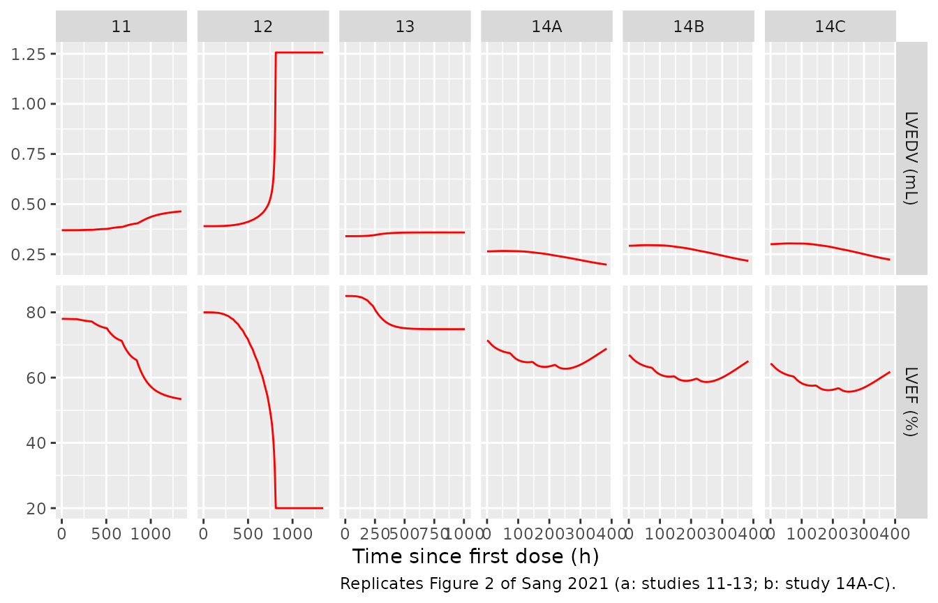
Study 11 is the panel with the largest change. The end-of-study values of its Figure 2 curve were read from the figure by the maintainers.
s11 <- rat_sim[rat_sim$study == "11" & rat_sim$time == 1344, ]
fig2_tab <- data.frame(
  Quantity = c("LVEF at 1344 h (%)", "LVEDV at 1344 h (mL)"),
  Simulated = round(c(s11$LVEF, s11$LVEDV), 3),
  "Figure 2a (read from curve)" = c(54.6, 0.458),
  check.names = FALSE
)
knitr::kable(fig2_tab)| Quantity | Simulated | Figure 2a (read from curve) |
|---|---|---|
| LVEF at 1344 h (%) | 53.405 | 54.600 |
| LVEDV at 1344 h (mL) | 0.464 | 0.458 |
The in-house groups can be compared with the observed Table S2 means (n = 9 per group) at days 4, 8 and 15.
obs_s2 <- data.frame(
  study = rep(c("14A", "14B", "14C"), each = 3),
  day = rep(c(4, 8, 15), 3),
  lvef_obs = c(63.8, 65.2, 77.1, 62.2, 56.6, 68.3, 59.8, 58.3, 61.7),
  lvef_sd = c(4.3, 3.3, 7.4, 3.9, 4.4, 8.5, 3.4, 4.5, 6.3),
  lvedv_obs = c(261.0, 242.0, 242.4, 288.2, 271.2, 240.2, 307.8, 307.1, 253.4) / 1000
)
pred_s2 <- rat_sim |>
  dplyr::filter(study %in% obs_s2$study, time %in% c(96, 192, 360)) |>
  dplyr::mutate(day = time / 24) |>
  dplyr::select(study, day, lvef_pred = LVEF, lvedv_pred = LVEDV)
s2_cmp <- dplyr::inner_join(obs_s2, pred_s2, by = c("study", "day"))
stopifnot(nrow(s2_cmp) == 9L)
s2_cmp |>
  dplyr::mutate(lvef_pred = round(lvef_pred, 1), lvedv_pred = round(lvedv_pred, 3)) |>
  dplyr::rename("Group" = study, "Day" = day, "LVEF obs (%)" = lvef_obs, "LVEF SD" = lvef_sd,
                "LVEF pred (%)" = lvef_pred, "LVEDV obs (mL)" = lvedv_obs,
                "LVEDV pred (mL)" = lvedv_pred) |>
knitr::kable()| Group | Day | LVEF obs (%) | LVEF SD | LVEDV obs (mL) | LVEF pred (%) | LVEDV pred (mL) |
|---|---|---|---|---|---|---|
| 14A | 4 | 63.8 | 4.3 | 0.2610 | 65.6 | 0.265 |
| 14A | 8 | 65.2 | 3.3 | 0.2420 | 63.3 | 0.250 |
| 14A | 15 | 77.1 | 7.4 | 0.2424 | 67.4 | 0.204 |
| 14B | 4 | 62.2 | 3.9 | 0.2882 | 61.2 | 0.294 |
| 14B | 8 | 56.6 | 4.4 | 0.2712 | 59.1 | 0.278 |
| 14B | 15 | 68.3 | 8.5 | 0.2402 | 63.6 | 0.223 |
| 14C | 4 | 59.8 | 3.4 | 0.3078 | 58.5 | 0.303 |
| 14C | 8 | 58.3 | 4.5 | 0.3071 | 56.2 | 0.287 |
| 14C | 15 | 61.7 | 6.3 | 0.2534 | 60.3 | 0.230 |
lvef_z <- (s2_cmp$lvef_pred - s2_cmp$lvef_obs) / s2_cmp$lvef_sd
stopifnot(median(abs(lvef_z)) < 1, all(abs(lvef_z) < 2.5))
The typical curve tracks the day-4 and day-8 nadir; the day-15 observations recover further than the model in the healthy group 14A, as the Figure 2b curve also shows.
Human model
Rat-to-human scaling (Table 1)
scale_f <- (0.25 / 70)^0.25
scaling <- data.frame(
  Parameter = c("kout_SV", "kout_LVEDV", "kout_HR", "kout_TPR", "FB_LVESV"),
  Rat = c(0.126, 0.126, 11.58, 3.58, 1.43),
  Recomputed = c(0.126 * scale_f, 0.126 * scale_f, 11.58 * scale_f, 3.58 * scale_f,
                 1.43 * 0.085 / (113 - 65)),
  "Table 1 human" = c(0.0308, 0.0308, 2.83, 0.875, 2.532e-3),
  check.names = FALSE
)
knitr::kable(scaling, digits = 5)| Parameter | Rat | Recomputed | Table 1 human |
|---|---|---|---|
| kout_SV | 0.126 | 0.03080 | 0.03080 |
| kout_LVEDV | 0.126 | 0.03080 | 0.03080 |
| kout_HR | 11.580 | 2.83086 | 2.83000 |
| kout_TPR | 3.580 | 0.87517 | 0.87500 |
| FB_LVESV | 1.430 | 0.00253 | 0.00253 |
Pre-treatment steady state
mod_hum <- readModelDb("Sang_2021_doxorubicin_human_qsp")
mod_hum_typ <- rxode2::zeroRe(rxode2::rxode2(mod_hum))

hum_ss <- data.frame(
  id = rep(1:2, each = 3), time = rep(c(0, 240, 2400), 2), evid = 0L, amt = 0, dvid = 1L,
  CEFFECT = 0, LVEDV_BL = rep(c(113, 141), each = 3), LVESV_BL = rep(c(48, 76), each = 3),
  HR_BL = 70, MAP_BL = rep(c(70 * 0.02 * 65, 70 * 0.025 * 65), each = 3)
)
hs <- rxode2::rxSolve(mod_hum_typ, hum_ss, returnType = "data.frame")
hs[, c("id", "time", "LVEF", "LVEDV", "LVESV", "MAP")]
#>   id time     LVEF LVEDV LVESV    MAP
#> 1  1    0 57.52212   113    48  91.00
#> 2  1  240 57.52212   113    48  91.00
#> 3  1 2400 57.52212   113    48  91.00
#> 4  2    0 46.09929   141    76 113.75
#> 5  2  240 46.09929   141    76 113.75
#> 6  2 2400 46.09929   141    76 113.75
stopifnot(max(abs(hs$LVEDV / rep(c(113, 141), each = 3) - 1)) < 1e-6,
          max(abs(hs$MAP / rep(c(91, 113.75), each = 3) - 1)) < 1e-6)
Figure 4: sensitivity to baseline LVEDV and MAP
Figure 4 plots the relative change of LVEF from baseline over about 11 months of 3-weekly doxorubicin for patients insensitive (AUC50_EP = 1390 ugh/mL, panels a-c) and sensitive (AUC50_EP = 463.3 ugh/mL, one third, panels d-f) to doxorubicin, varying baseline LVEDV and MAP. The floor of -65.2% in panels d and e (LVEF frozen at 20% by the model’s numerical guard) shows that baseline LVEF was held at 65/113 = 57.5% as LVEDV was varied.
The heart-concentration profile came from the He 2018 PBPK model and is not reproduced here. Because the turnover states equilibrate within days, the late plateau of Figure 4 depends on the final cumulative heart AUC and not on the shape of the profile, so an illustrative driver is used: nine 24-hour constant-concentration pulses, 21 days apart. Its total AUC is calibrated so that the reference curve of panel d (LVEDV 113 mL, MAP 91 mmHg) ends at the digitised -31.9%; every other curve is then a prediction.
fig4_events <- function(auc_total, lvedv, map, id = 1L) {
  starts <- (0:8) * 21 * 24
  tt <- sort(unique(c(seq(0, 330 * 24, by = 24), starts, starts + 24)))
  on <- vapply(tt, function(t) any(t >= starts & t < starts + 24), logical(1))
  sv <- lvedv * 65 / 113
  data.frame(id = id, time = tt, evid = 0L, amt = 0, dvid = 1L,
             CEFFECT = ifelse(on, auc_total / (9 * 24), 0),
             LVEDV_BL = lvedv, LVESV_BL = lvedv - sv, HR_BL = 70, MAP_BL = map)
}
lvef_change <- function(auc_total, auc50, lvedv, map) {
  m <- mod_hum_typ |> rxode2::ini(lauc50_ep = log(auc50))
  s <- rxode2::rxSolve(m, fig4_events(auc_total, lvedv, map), covsInterpolation = "locf",
                       returnType = "data.frame", maxsteps = 1e6)
  s$change <- 100 * (s$LVEF / (65 / 113 * 100) - 1)
  s
}
auc_cal <- uniroot(function(a) tail(lvef_change(a, 463.3, 113, 91)$change, 1) + 31.9,
                   c(200, 1000), tol = 1e-3)$root
auc_cal
#> [1] 435.5382

fig4_cases <- dplyr::bind_rows(
  data.frame(panel = "a", auc50 = 1390, lvedv = c(113, 130, 146, 163, 180), map = c(91, 104, 118, 131, 145),
             digitised = c(-2.47, -2.68, -2.93, -3.20, -3.60)),
  data.frame(panel = "b", auc50 = 1390, lvedv = c(113, 130, 146, 163, 180), map = 91,
             digitised = c(-2.47, -2.65, -2.84, -3.02, -3.29)),
  data.frame(panel = "c", auc50 = 1390, lvedv = 113, map = c(91, 106, 120, 135, 150),
             digitised = c(-2.47, NA, NA, NA, -2.68)),
  data.frame(panel = "d", auc50 = 463.3, lvedv = c(113, 130, 146, 163, 180), map = c(91, 104, 118, 131, 145),
             digitised = c(-31.9, -34.1, -36.8, -41.3, -65.2)),
  data.frame(panel = "e", auc50 = 463.3, lvedv = c(113, 130, 146, 163, 180), map = 91,
             digitised = c(-31.9, -33.3, -35.4, -38.6, -65.2)),
  data.frame(panel = "f", auc50 = 463.3, lvedv = 113, map = c(91, 106, 120, 135, 150),
             digitised = c(-31.9, NA, NA, NA, -34.6))
)
fig4_sim <- dplyr::bind_rows(lapply(seq_len(nrow(fig4_cases)), function(i) {
  cs <- fig4_cases[i, ]
  s <- lvef_change(auc_cal, cs$auc50, cs$lvedv, cs$map)
  data.frame(panel = cs$panel, curve = sprintf("LVEDV = %g, MAP = %g", cs$lvedv, cs$map),
             day = s$time / 24, change = s$change, auc_heart = s$auc_heart)
}))

ggplot(fig4_sim, aes(day, change, colour = curve)) +
  geom_line() +
  facet_wrap(~panel, scales = "free_y") +
  labs(x = "Time since enrollment (day)", y = "LVEF change from baseline (%)", colour = NULL,
       caption = "Replicates Figure 4 of Sang 2021 with an illustrative heart-exposure driver.") +
  theme(legend.position = "bottom")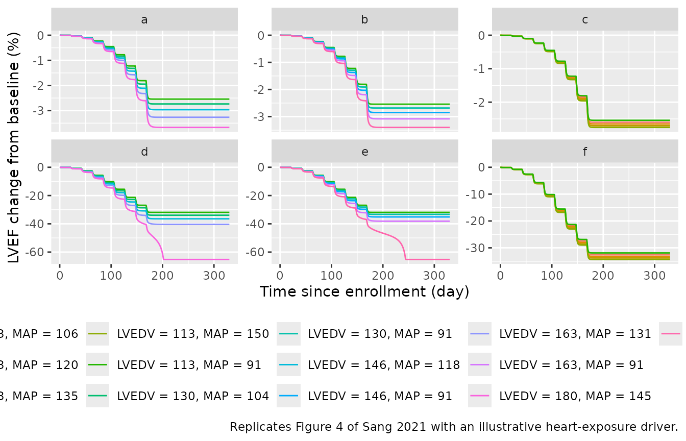
plateau <- fig4_sim |>
  dplyr::group_by(panel, curve) |>
  dplyr::summarise(simulated = dplyr::last(change), auc_end = dplyr::last(auc_heart), .groups = "drop")
# Every curve must have integrated the whole driver: a covariate supplied on too
# sparse a time grid is stepped over by the solver and silently lost.
stopifnot(all(abs(plateau$auc_end / auc_cal - 1) < 1e-3))
fig4_cmp <- fig4_cases |>
  dplyr::mutate(curve = sprintf("LVEDV = %g, MAP = %g", lvedv, map)) |>
  dplyr::inner_join(plateau, by = c("panel", "curve"))
stopifnot(nrow(fig4_cmp) == nrow(fig4_cases))
fig4_cmp |>
  dplyr::filter(!is.na(digitised)) |>
  dplyr::mutate(simulated = round(simulated, 2)) |>
  dplyr::select("Panel" = panel, "Baselines" = curve, "Figure 4 plateau (%)" = digitised,
                "Simulated (%)" = simulated) |>
knitr::kable()| Panel | Baselines | Figure 4 plateau (%) | Simulated (%) |
|---|---|---|---|
| a | LVEDV = 113, MAP = 91 | -2.47 | -2.54 |
| a | LVEDV = 130, MAP = 104 | -2.68 | -2.74 |
| a | LVEDV = 146, MAP = 118 | -2.93 | -2.97 |
| a | LVEDV = 163, MAP = 131 | -3.20 | -3.27 |
| a | LVEDV = 180, MAP = 145 | -3.60 | -3.67 |
| b | LVEDV = 113, MAP = 91 | -2.47 | -2.54 |
| b | LVEDV = 130, MAP = 91 | -2.65 | -2.68 |
| b | LVEDV = 146, MAP = 91 | -2.84 | -2.85 |
| b | LVEDV = 163, MAP = 91 | -3.02 | -3.08 |
| b | LVEDV = 180, MAP = 91 | -3.29 | -3.40 |
| c | LVEDV = 113, MAP = 91 | -2.47 | -2.54 |
| c | LVEDV = 113, MAP = 150 | -2.68 | -2.76 |
| d | LVEDV = 113, MAP = 91 | -31.90 | -31.90 |
| d | LVEDV = 130, MAP = 104 | -34.10 | -33.92 |
| d | LVEDV = 146, MAP = 118 | -36.80 | -36.46 |
| d | LVEDV = 163, MAP = 131 | -41.30 | -40.40 |
| d | LVEDV = 180, MAP = 145 | -65.20 | -65.23 |
| e | LVEDV = 113, MAP = 91 | -31.90 | -31.90 |
| e | LVEDV = 130, MAP = 91 | -33.30 | -33.32 |
| e | LVEDV = 146, MAP = 91 | -35.40 | -35.13 |
| e | LVEDV = 163, MAP = 91 | -38.60 | -38.15 |
| e | LVEDV = 180, MAP = 91 | -65.20 | -65.23 |
| f | LVEDV = 113, MAP = 91 | -31.90 | -31.90 |
| f | LVEDV = 113, MAP = 150 | -34.60 | -34.33 |
chk <- fig4_cmp[!is.na(fig4_cmp$digitised), ]
stopifnot(nrow(chk) == 24L, all(abs(chk$simulated - chk$digitised) < 1.5))
A single calibrated exposure reproduces every digitised plateau within about one percentage point, including the ordering across baselines, the small MAP effect (panels c and f) and the 20% LVEF floor.
Figure S5: sensitivity to AUC50_EP
Figure S5 varies AUC50_EP over a nine-fold range for the typical healthy patient (LVEDV 113 mL, MAP 91 mmHg). With the same calibrated exposure:
s5 <- data.frame(auc50 = c(463.3, 802.5, 1390, 2407),
                 digitised = c(-32.2, -10.8, -2.65, -0.6))
s5$simulated <- vapply(s5$auc50, function(a) tail(lvef_change(auc_cal, a, 113, 91)$change, 1),
                       numeric(1))
s5 |>
  dplyr::mutate(simulated = round(simulated, 2)) |>
  dplyr::rename("AUC50_EP (ug*h/mL)" = auc50, "Figure S5 plateau (%)" = digitised,
                "Simulated (%)" = simulated) |>
knitr::kable()| AUC50_EP (ug*h/mL) | Figure S5 plateau (%) | Simulated (%) |
|---|---|---|
| 463.3 | -32.20 | -31.90 |
| 802.5 | -10.80 | -11.16 |
| 1390.0 | -2.65 | -2.54 |
| 2407.0 | -0.60 | -0.51 |
The Results text says LVEF reduction “increased from 5% to 32%” as AUC50_EP fell from 1390 to 463.3; the Figure S5 and Figure 4 curves show about 2.5% at 1390, which the model reproduces.
Virtual cohort (illustrative)
The published incidence curves (Figure 3) need the He 2018 heart
exposure and cannot be reproduced here. The chunk below shows how a
virtual cohort is set up: baselines vary log-normally with 30% CV around
the Table 1 typical values (healthy: SV 65 mL, LVEDV 113 mL, HR 70
beats/min, TPR 0.02 mmHg*min/mL; diseased: LVEDV 141 mL and TPR 0.025),
with the Table 1 variability on FB_LVESV and AUC50_EP. Draws whose
baseline LVEF falls outside 35-80% are redrawn. The driver is the same
illustrative pulse train, at the calibrated total heart AUC, supplied on
a daily grid: rxode2 does not restart the integrator where a covariate
changes, so a CEFFECT profile given only at its change
points can be stepped over and lost. The chunk checks that every patient
accumulated the full heart AUC.
rxode2::rxSetSeed(20210512)
set.seed(20210512)
draw_arm <- function(n, lvedv0, tpr0, arm, id0) {
  out <- data.frame()
  while (nrow(out) < n) {
    d <- data.frame(sv = 65 * exp(rnorm(n, 0, sqrt(log(1.09)))),
                    lvedv = lvedv0 * exp(rnorm(n, 0, sqrt(log(1.09)))),
                    hr = 70 * exp(rnorm(n, 0, sqrt(log(1.09)))),
                    tpr = tpr0 * exp(rnorm(n, 0, sqrt(log(1.09)))))
    d <- d[d$sv / d$lvedv > 0.35 & d$sv / d$lvedv < 0.80, ]
    out <- rbind(out, d)
  }
  out <- out[seq_len(n), ]
  out$id <- id0 + seq_len(n)
  out$arm <- arm
  out
}
pts <- rbind(draw_arm(100, 113, 0.020, "Cardiovascular healthy", 0L),
             draw_arm(100, 141, 0.025, "Cardiovascular disease", 100L))
cohort_events <- dplyr::bind_rows(lapply(seq_len(nrow(pts)), function(i) {
  p <- pts[i, ]
  e <- fig4_events(auc_cal, p$lvedv, p$hr * p$tpr * p$sv, id = p$id)
  e$LVESV_BL <- p$lvedv - p$sv
  e$HR_BL <- p$hr
  e$arm <- p$arm
  e
}))
cohort <- rxode2::rxSolve(mod_hum, cohort_events, keep = "arm", covsInterpolation = "locf",
                          returnType = "data.frame", maxsteps = 1e6)
cohort_end <- cohort |>
  dplyr::group_by(id, arm) |>
  dplyr::summarise(change = 100 * (dplyr::last(LVEF) / dplyr::first(LVEF) - 1),
                   auc_end = dplyr::last(auc_heart), .groups = "drop")
cohort_end |>
  dplyr::group_by(arm) |>
  dplyr::summarise(N = dplyr::n(), median_change = median(change),
                   pct_ge_10pct_decline = 100 * mean(change <= -10)) |>
  dplyr::rename("Arm" = arm, "Median LVEF change (%)" = median_change,
                "Patients with >= 10% decline (%)" = pct_ge_10pct_decline) |>
knitr::kable(digits = 1)| Arm | N | Median LVEF change (%) | Patients with >= 10% decline (%) |
|---|---|---|---|
| Cardiovascular disease | 100 | -2.9 | 1 |
| Cardiovascular healthy | 100 | -2.6 | 1 |
Assumptions and deviations
- Units. Table S4 prints the PK volumes as L/kg and Tables 1 and S5 print AUC50 in mgh/mL. The deposited code only reproduces Figure S2 (ng/mL axes) when the dose is a per-animal amount and the volumes are per-animal mL, and it only reproduces the gradual Figure 2 decline when that amount is in ug (in ng the bioenergy effect saturates at the first dose and LVEF collapses to the 20% floor). The models therefore use per-animal ug doses, mL volumes, ug/mL concentrations and AUC50 in ugh/mL (numerically mgh/L). Heart rate is in beats/min although the tables print beats/h; the model is unaffected because TPR is derived from MAP / (HR SV).
-
PK values. The model uses the as-run Mlxtran
constants. Table S4 labels the plasma-heart exchange
k_in_heart/k_out_heartand the two peripheral pairsk12/k21andk13/k31, matching the code’sK12/K21,K13/K31andK14/K41. Table S4 prints the slow return rate as 0.0586 1/h; the code uses 0.0568 1/h, which is kept because it is the value the QSP parameters were estimated against. ka is 4.532 (code) versus 4.53 (Table S4). -
Strain switch. The code’s
Speciesregressor removes the myocardial-compliance effect (EdrugMC * (1 - Species), commented “Wistar”). It is encoded asSTRAIN_SD(1 = Sprague-Dawley), because studies 11-13 were Sprague-Dawley rats with the systolic-dysfunction phenotype of Figure 2a and study 14A-C used WKY / SHR rats with the diastolic phenotype of Figure 2b. - Numerical guard and feedback clamp. The deposited code freezes all four turnover states once SV or LVESV is non-positive or LVEF is at or below 20%, and clamps the MAP feedback term at 1 for HR, TPR and LVEDV but not for SV. Both are reproduced as coded, in the human model too.
- Reference MAP of Eq. 8. The code uses MAP_0 = 106.596 mmHg (the typical rat MAP). Table 1 does not list MAP_0 among the rescaled parameters, so the human model keeps 106.596. Replacing it with the human typical 91 mmHg moves the Figure 4 plateaus by at most 0.5 percentage points, so the figure cannot distinguish the two readings.
-
Human model scope. Only the bioenergy-production
(systolic) effect is translated, as stated in the Methods and reflected
in Table 1, which lists AUC50_EP but not AUC50_MC or kt. The human
heart-tissue concentration must be supplied as
CEFFECTfrom an external PK model; Sang 2021 used He 2018 (Pharm Res 35:174), which is not in nlmixr2lib. - Human variability. The Table 1 CV column gives 12.4% for FB_LVESV and 7.06% for AUC50_EP, the rat relative standard errors of those estimates. They are encoded as log-normal between-patient variability (variance log(1 + CV^2)) and held fixed. The 30% variability on the baselines is not in the model because the baselines are covariates; the virtual cohort above samples them log-normally, and the redraw window for baseline LVEF (35-80%) is the maintainers’ choice, as the paper does not state how implausible draws were handled.
- Table 1 “65/115”. The SV0 row reads “65/115” for healthy/diseased. A diseased SV of 115 mL with LVEDV 141 mL would give LVEF 82% and MAP 201 mmHg; with SV 65 mL, TPR 0.025 and HR 70 the diseased MAP is 113.75 mmHg, close to the 115 mmHg hypertension threshold. The cohort above keeps SV at 65 mL for both arms.
- Residual error. Supplementary Methods name additive error for LVEF and MAP and proportional error for LVEDV and LVESV but report no estimates; they are fixed to 0. No between-animal variability was reported for the rat model.
- Study schedules. Figure 2b shows six dose arrows for study 14, whereas Table S1 and the Supplementary Methods give four doses every 3 days; the latter is used. Schedules for studies 11-13 are read from the Figure 2a arrows.