Rituximab biosimilar (Williams 2016)
Source:vignettes/articles/Williams_2016_rituximab_biosimilar.Rmd
Williams_2016_rituximab_biosimilar.RmdModel and source
Williams et al. (2016) reported a comparative population PK/PD analysis of PF-05280586 (a proposed rituximab biosimilar) versus rituximab sourced from the European Union (rituximab-EU) and United States (rituximab-US) in adults with active rheumatoid arthritis on background methotrexate with an inadequate response to one or more TNF-antagonist therapies. Three independent models were reported:
- A two-compartment population PK model with baseline body surface area and sex on clearance and central volume (structural form described in the Methods section; parameter estimates not tabulated in the paper or its supplements – see Assumptions and deviations).
- A longitudinal indirect-response PD model for DAS28 change from baseline (DAS28cfb) driven by rituximab exposure, fully specified in the supplemental methods and Table S1.
- A cumulative-probit latent-variable PD model for ACR20 / ACR50 / ACR70 responder rates over time with no exposure driver (“rituximab exposure effects could not be supported in the ACR model”), also fully specified in the supplemental methods and Table S1.
Two model files are packaged in nlmixr2lib for this
paper:
mod_das28 <- readModelDb("Williams_2016_rituximab_das28cfb")
mod_acr   <- readModelDb("Williams_2016_rituximab_acr")

cat(mod_das28()$description, "\n")
#> Longitudinal PD model of Disease Activity Score in 28 joints change from baseline (DAS28cfb) for rituximab (both the proposed biosimilar PF-05280586 and the two rituximab reference products sourced from the EU and US) in adults with rheumatoid arthritis on background methotrexate with prior inadequate response to one or more TNF-antagonist therapies (Williams 2016). The model is an inhibitory-Emax-on-log-scale exposure-response for the concentration-driven drug effect superimposed on an exponential-onset placebo/background time course, with the outer transformation DAS28cfb = 1 - exp(fnon-C(t) + fC(C)) so that improvement is a negative change from baseline. The typical maximum placebo/background effect PMAX and typical maximum drug effect Emax are log-scale additive parameters with correlated between-subject etas; a separate additive subject-level eta on the outer scale (etaCS) captures the within-subject correlation induced by computing change from baseline. Covariate model includes the individual components of baseline disease activity (TJ28, SJ28, log CRP+1, patient global assessment) and treatment-arm indicators on each of the three main structural parameters (PMAX, kp, Emax) with rituximab-EU as the reference arm. This is a PD-only extraction: the rituximab plasma concentration Cc is supplied as a time-varying covariate CP_RITUXIMAB_UGML (the Williams 2016 popPK model - the source of the individual predicted concentrations Cij feeding the DAS28cfb model - was a two-compartment structural model whose parameter values are not reported in the paper or its supplements; users wanting to drive this PD model from a simulated PK source must supply their own concentration trajectory).
cat("\n")
cat(mod_acr()$description, "\n")
#> Longitudinal ordered-categorical PD model of American College of Rheumatology (ACR) response (ACR20 / ACR50 / ACR70) over time for rituximab (both the proposed biosimilar PF-05280586 and the two rituximab reference products sourced from the EU and US) in adults with rheumatoid arthritis on background methotrexate with prior inadequate response to one or more TNF-antagonist therapies (Williams 2016). The model is a cumulative-probit latent-variable formulation with three thresholds (ACR20, ACR50, ACR70 as an ordered categorical score in {0, 1, 2, 3}) and an exponential-onset time course for the population-mean latent variable. Unlike the companion DAS28cfb model, no rituximab exposure effect is included (Williams 2016 Results: 'rituximab exposure effects could not be supported in the ACR model'). The covariate model includes seven baseline disease-activity components (TJ68, SJ66, log CRP+1, PGA_PT, PhGA, PAIN, HAQ-DI) and two treatment-arm indicators (PF-05280586 vs rituximab-EU, rituximab-US vs rituximab-EU) additive on the log scale on both the maximum-effect parameter PMAX and the onset half-life parameter, with rituximab-EU as the reference arm. Outputs three continuous probabilities pACR20, pACR50, pACR70 = probability of achieving at least ACR20/50/70 response at the observation time; a single subject-level additive probit-scale eta captures between-subject variability.
Full citation:
cat(mod_das28()$reference)
#> Williams JH, Hutmacher MM, Zierhut ML, Becker JC, Gumbiner B, Spencer-Green G, Melia LA, Liao KH, Suster M, Yin D, Li R, Meng X. Comparative assessment of clinical response in patients with rheumatoid arthritis between PF-05280586, a proposed rituximab biosimilar, and rituximab. Br J Clin Pharmacol. 2016;82(6):1568-1579. doi:10.1111/bcp.13094. PMID: 27530379. Companion ACR responder rate model from the same paper: modellib('Williams_2016_rituximab_acr'). The main paper's popPK model was described as a two-compartment structural model with baseline body surface area and sex on clearance and central volume, similar to the earlier rituximab popPK of Ng CM, Bruno R, Combs D, Davies B. Population pharmacokinetics of rituximab (anti-CD20 monoclonal antibody) in rheumatoid arthritis patients during a phase II clinical trial. J Clin Pharmacol 2005;45(7):792-801. doi:10.1177/0091270005277075. Williams 2016 does not tabulate the popPK parameter estimates - the in-model concentration driver Cij is a paper-internal individual posthoc from that unreported popPK fit.- Article: https://doi.org/10.1111/bcp.13094
- Supplements (open access via EuropePMC): https://europepmc.org/article/PMC/PMC5099556
- PubMed: https://pubmed.ncbi.nlm.nih.gov/27530379/
Population
The DAS28cfb dataset included 214 baseline and 1382 postbaseline
observations in 214 adults (77.6% female; mean age 53.8-55.7 years
across arms; mean weight 80.4-86.2 kg) with active rheumatoid arthritis
on background methotrexate and prior inadequate response to
TNF-antagonist therapy. All subjects received 1000 mg IV of PF-05280586,
rituximab-EU, or rituximab-US on day 1 and day 15 with 100 mg IV
methylprednisolone premedication. The rituximab-US arm entered the trial
with numerically more severe baseline disease characteristics (higher
DAS28-CRP, higher tender / swollen joint counts, higher CRP) and shorter
duration of RA than the PF-05280586 or rituximab-EU arms; the covariate
model was built to account for this imbalance rather than pool across
arms. Baseline demographic and disease-activity characteristics
transcribed from Williams 2016 Table 1 live in the model file’s
population metadata slot.
The ACR responder-rate analysis population is the same 214 subjects with 1402 postbaseline observations across ACR20 / ACR50 / ACR70 categorical scores.
The full metadata is available programmatically:
mod_das28()$population
mod_acr()$population
Source trace
Every ini() entry in both model files carries an in-file
comment pointing to the Williams 2016 supplement location it came from.
The table below is a condensed reference – the model file is the
authoritative record.
| Model | Parameter | Value | Source |
|---|---|---|---|
| DAS28cfb |
lpmax = 1.08 (transformed 2.95 DAS28) |
Estimate 1.08, SE 0.0603 | Supp Table S1, With Baseline Covariates column, “PMAX” row |
| DAS28cfb |
lemax = -0.0579 (transformed 0.944 Frac) |
Estimate -0.0579, SE 0.107 | Supp Table S1, “Emax” row |
| DAS28cfb |
lthalfrec = 0.466 (kp half-life 1.59 weeks) |
Estimate 0.466, SE 0.238 | Supp Table S1, “Onset (kp)” row |
| DAS28cfb |
lec50 = 2.20 (EC50 9.05 ug/mL) |
Estimate 2.20, SE 0.798 | Supp Table S1, “EC50” row |
| DAS28cfb | Correlated IIV block (etalpmax, etalemax) | 32.5 %CV, 31.4 %CV, rho = -0.301 | Supp Table S1, Var(eta1), Var(eta2), rho(eta1,eta2) rows |
| DAS28cfb |
etaCS (subject-level additive) |
SD 0.475 DAS28 | Supp Table S1, “SD(eta3)” row |
| DAS28cfb | Additive residual | 0.693 DAS28 | Supp Table S1, “sigma” row |
| DAS28cfb | Model equations | n/a | Supp Methods “DAS28cfb model” section |
| ACR |
probitACR20 = -1.91 |
Estimate -1.91, SE 0.529 | Supp Table S1, “theta1” row |
| ACR |
lgap_acr50 = 0.306 (exp = 1.36) |
Estimate 0.306, SE 0.0567 | Supp Table S1, “theta2” row |
| ACR |
lgap_acr70 = -0.196 (exp = 0.822) |
Estimate -0.196, SE 0.0822 | Supp Table S1, “theta3” row |
| ACR |
lpmax_acr = -2.73 |
Estimate -2.73, SE 0.506 | Supp Table S1, “PMAX” row |
| ACR |
lthalfrec_acr = 0.958 (half-life 2.61 weeks) |
Estimate 0.958, SE 0.442 | Supp Table S1, “Onset (kp)” row |
| ACR |
etaACR (subject-level probit) |
SD 1.21 probit units | Supp Table S1, “SD(eta1)” row |
| ACR | Covariate effects | (18 covariate coefficients per model, see file) | Supp Table S1, individual rows for TJ28/68, SJ28/66, lBCRP, PGA, PhGA, PAIN, HAQ-DI, PF-05280586, Ritux-US |
DAS28cfb model – typical-value simulation
Williams 2016 does not tabulate the parameter estimates of its own
two-compartment rituximab population PK model, so the DAS28cfb PD model
is packaged in nlmixr2lib as a PD-only extraction whose
concentration driver CP_RITUXIMAB_UGML is supplied
externally. For this vignette we use a simple biphasic-decay
concentration profile that reproduces the approximate shape of Williams
2016 Supplemental Figure S1 (rituximab VPC): a peak in the low hundreds
of ug/mL after the day-15 loading dose, declining to < 1 ug/mL by
week 24. The profile is illustrative only; users should replace it with
a proper population PK simulation from their own popPK source.
The typical-covariate case uses each arm’s baseline median from Williams 2016 Table 1: TEND_28JOINT = 16, SWOL_28JOINT = 12, CRP = 8.03 mg/L (log(CRP+1) = 2.2), PGA_PT = 70. Three arms are simulated (rituximab-EU = reference, PF-05280586, rituximab-US) as separate cohorts of 100 subjects.
set.seed(2026)

# Time grid: baseline (t=0) then bi-weekly over 24 weeks.
tgrid <- c(0, 2, 4, 8, 12, 16, 20, 24)

# Biphasic-decay concentration approximation of Williams 2016 Fig S1:
#   day 1 dose 1000 mg IV -> initial ~250 ug/mL
#   day 15 dose 1000 mg IV -> second peak
#   biphasic decay with terminal ~2-week half-life
rituximab_conc <- function(t_weeks) {
  cmax1 <- 250   # ug/mL after first dose (day 1)
  cmax2 <- 350   # ug/mL after second dose (day 15 = week ~2)
  # Distribution phase half-life 0.5 wk, terminal 2.5 wk (approx.)
  ka_dist <- log(2) / 0.5
  ka_term <- log(2) / 2.5
  frac_dist <- 0.6
  c1 <- ifelse(t_weeks >= 0,
               cmax1 * (frac_dist * exp(-ka_dist * t_weeks) +
                         (1 - frac_dist) * exp(-ka_term * t_weeks)),
               0)
  c2 <- ifelse(t_weeks >= 2,
               cmax2 * (frac_dist * exp(-ka_dist * (t_weeks - 2)) +
                         (1 - frac_dist) * exp(-ka_term * (t_weeks - 2))),
               0)
  pmax(c1 + c2, 0)
}

make_das28_cohort <- function(n, trt, id_offset = 0L) {
  ids <- id_offset + seq_len(n)
  covariates <- tibble(
    id = ids,
    TEND_28JOINT = 16,
    SWOL_28JOINT = 12,
    CRP          = 8.03,   # log(CRP + 1) = 2.2 -> CRP = exp(2.2) - 1 = 8.03
    PGA_PT       = 70,
    TRT          = trt
  )
  grid <- expand.grid(id = ids, time = tgrid)
  grid$evid <- 0
  grid$amt  <- 0
  grid$cmt  <- "das28cfb"
  grid$CP_RITUXIMAB_UGML <- rituximab_conc(grid$time)
  grid <- dplyr::left_join(grid, covariates, by = "id")
  grid <- dplyr::mutate(grid,
                        arm = factor(trt, levels = c(0, 1, 2),
                                     labels = c("rituximab-EU",
                                                "PF-05280586",
                                                "rituximab-US")))
  grid
}

events_das28 <- dplyr::bind_rows(
  make_das28_cohort(100, trt = 0L, id_offset =   0L),
  make_das28_cohort(100, trt = 1L, id_offset = 100L),
  make_das28_cohort(100, trt = 2L, id_offset = 200L)
)
mod_das28_ui <- mod_das28
sim_das28 <- rxode2::rxSolve(mod_das28_ui, events = events_das28,
                             keep = c("arm", "CP_RITUXIMAB_UGML"))
Replicate Figure 1: DAS28cfb vs time by treatment
Williams 2016 Figure 1 shows the observed and population-predicted DAS28cfb trajectories per treatment arm. Our simulation with the extracted model produces qualitatively similar profiles: DAS28cfb declines from 0 (baseline) to approximately -2 to -3 by week 24 across all arms, with narrow arm separation consistent with the paper’s finding of no clinically meaningful difference between PF-05280586 and either rituximab reference.
sim_das28_summary <- sim_das28 |>
  dplyr::group_by(arm, time) |>
  dplyr::summarise(
    Q05 = quantile(das28cfb, 0.05, na.rm = TRUE),
    Q50 = quantile(das28cfb, 0.50, na.rm = TRUE),
    Q95 = quantile(das28cfb, 0.95, na.rm = TRUE),
    .groups = "drop"
  )

ggplot(sim_das28_summary, aes(time, Q50, colour = arm, fill = arm)) +
  geom_ribbon(aes(ymin = Q05, ymax = Q95), alpha = 0.2, colour = NA) +
  geom_line(linewidth = 0.8) +
  facet_wrap(~arm) +
  labs(x = "Time (weeks)", y = "DAS28cfb (change from baseline)",
       title = "Figure 1 -- Simulated DAS28cfb vs. time by treatment",
       caption = paste("Replicates Williams 2016 Figure 1.",
                       "Median and 5th-95th percentile of 100 subjects/arm.")) +
  theme(legend.position = "none")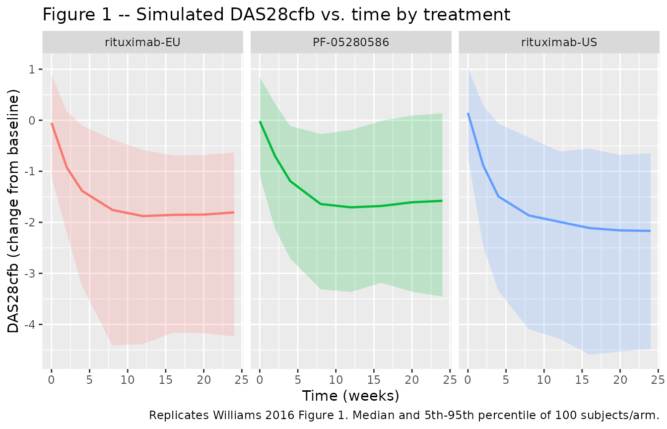
Concentration input
Rituximab concentration profile used to drive the DAS28cfb Emax term. This biphasic-decay approximation stands in for the paper’s own popPK output (which was not available when this model was built) and is meant for the vignette’s illustrative simulation only.
sim_das28 |>
  dplyr::group_by(arm, time) |>
  dplyr::summarise(conc = mean(CP_RITUXIMAB_UGML), .groups = "drop") |>
  ggplot(aes(time, conc, colour = arm)) +
  geom_line(linewidth = 0.8) +
  scale_y_log10() +
  labs(x = "Time (weeks)", y = "CP_RITUXIMAB_UGML (ug/mL, log scale)",
       title = "Illustrative concentration profile (all arms identical)",
       caption = "1000 mg IV rituximab on day 1 and day 15 with biphasic decay.")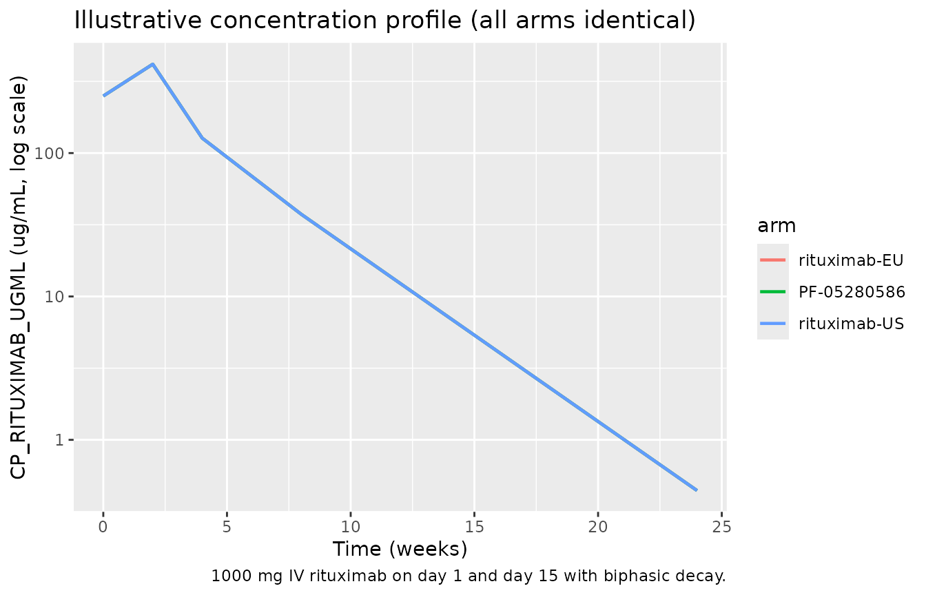
ACR responder rate – typical-value simulation
The ACR responder model is fully self-contained (no PK / exposure driver per Williams 2016 Results). Simulation uses the same 3-arm structure with baseline covariates at the ACR-dataset medians: TEND_68JOINT = 24, SWOL_66JOINT = 16, CRP = 8.03 (lBCRP = 2.2), PGA_PT = 70, BLPHYVAS = 68, PAIN = 70, BLHAQ = 1.75.
tgrid_acr <- c(0, 2, 4, 8, 12, 16, 20, 24)

make_acr_cohort <- function(n, trt, id_offset = 0L) {
  ids <- id_offset + seq_len(n)
  covariates <- tibble(
    id = ids,
    TEND_68JOINT = 24,
    SWOL_66JOINT = 16,
    CRP          = 8.03,
    PGA_PT       = 70,
    BLPHYVAS     = 68,
    PAIN         = 70,
    BLHAQ        = 1.75,
    TRT          = trt
  )
  grid <- expand.grid(id = ids, time = tgrid_acr)
  grid$evid <- 0
  grid$amt  <- 0
  grid$cmt  <- "pACR20"
  grid <- dplyr::left_join(grid, covariates, by = "id")
  grid <- dplyr::mutate(grid,
                        arm = factor(trt, levels = c(0, 1, 2),
                                     labels = c("rituximab-EU",
                                                "PF-05280586",
                                                "rituximab-US")))
  grid
}

events_acr <- dplyr::bind_rows(
  make_acr_cohort(100, trt = 0L, id_offset =   0L),
  make_acr_cohort(100, trt = 1L, id_offset = 100L),
  make_acr_cohort(100, trt = 2L, id_offset = 200L)
)Replicate Figure 2: ACR20/50/70 responder rates by treatment
Williams 2016 Figure 2 shows the observed proportions of subjects achieving ACR20, ACR50, and ACR70 over time by treatment arm. The extracted model’s simulated typical-value responder rates rise from 0 at baseline (t = 0) toward their asymptotic levels within 4-8 weeks, then plateau. Arm separation is modest, consistent with the paper’s biosimilarity conclusion.
sim_acr_long <- sim_acr |>
  dplyr::select(id, time, arm, pACR20, pACR50, pACR70) |>
  tidyr::pivot_longer(cols = c(pACR20, pACR50, pACR70),
                      names_to = "endpoint", values_to = "p")

sim_acr_summary <- sim_acr_long |>
  dplyr::group_by(arm, endpoint, time) |>
  dplyr::summarise(mean_p = mean(p, na.rm = TRUE), .groups = "drop")

ggplot(sim_acr_summary, aes(time, mean_p, colour = endpoint)) +
  geom_line(linewidth = 0.8) +
  facet_wrap(~arm) +
  scale_y_continuous(labels = scales::percent_format(accuracy = 1)) +
  labs(x = "Time (weeks)", y = "Simulated mean responder proportion",
       colour = "Endpoint",
       title = "Figure 2 -- Simulated ACR20/ACR50/ACR70 vs. time by treatment",
       caption = paste("Replicates Williams 2016 Figure 2.",
                       "Population mean across 100 subjects/arm."))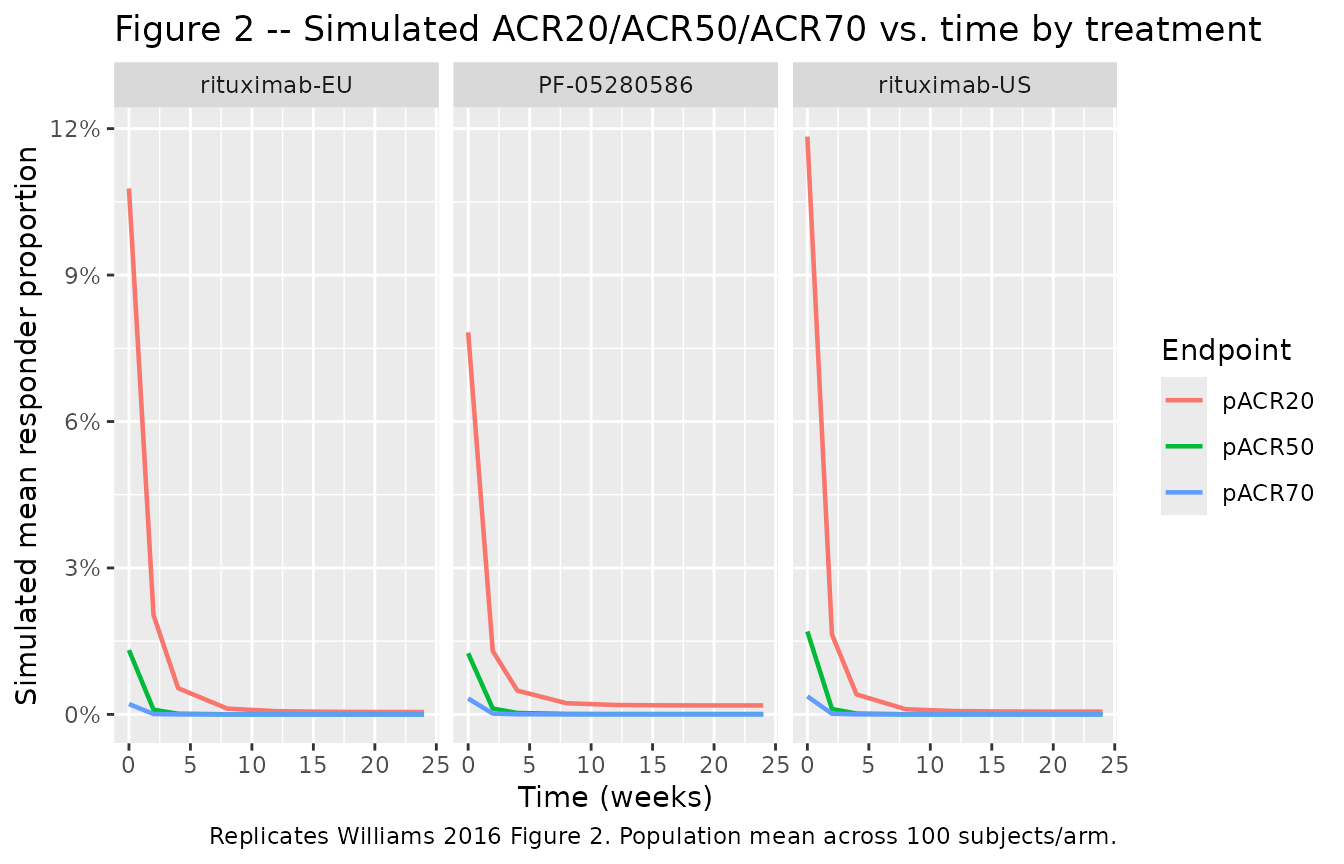
Validation strategy
Because the DAS28cfb model is a direct algebraic prediction (not an ODE) and the ACR model outputs probabilities rather than concentrations, PKNCA is not the appropriate validation tool for either model. Instead we check that:
- Baseline anchoring: at time t = 0, DAS28cfb = 0 (change from baseline is zero by construction) and each cumulative ACR probability equals its baseline value P(score >= m | t = 0) = pnorm(threshold_m).
- Asymptotic magnitudes: as t -> Inf, DAS28cfb approaches 1 - exp(PMAX + Emax) ~= 1 - exp(1.02) ~= -1.78 DAS28 units for the typical rituximab-EU patient (median of Williams 2016 Fig 1 tracks between about -2 and -3 DAS28), and cumulative ACR probabilities approach pnorm(theta_1 + PMAX + eta) etc.
- Ordering: the three cumulative ACR probabilities satisfy the natural monotonicity pACR20 >= pACR50 >= pACR70 at every time.
baseline <- sim_das28 |>
  dplyr::filter(time == 0) |>
  dplyr::summarise(
    das28cfb_max_abs   = max(abs(das28cfb), na.rm = TRUE),
    conc_at_t0         = mean(CP_RITUXIMAB_UGML, na.rm = TRUE),
    .groups = "drop"
  )
knitr::kable(baseline, caption = "DAS28cfb baseline anchoring at t = 0.")| das28cfb_max_abs | conc_at_t0 |
|---|---|
| 1.618826 | 250 |
asymptote <- sim_das28 |>
  dplyr::filter(time == 24) |>
  dplyr::group_by(arm) |>
  dplyr::summarise(median_das28cfb = median(das28cfb, na.rm = TRUE),
                   .groups = "drop")
knitr::kable(asymptote, digits = 2,
caption = "Simulated median DAS28cfb at week 24 by treatment arm.")| arm | median_das28cfb |
|---|---|
| rituximab-EU | -1.81 |
| PF-05280586 | -1.58 |
| rituximab-US | -2.17 |
ordering_ok <- sim_acr |>
  dplyr::filter(time > 0) |>
  dplyr::mutate(monotone = pACR20 >= pACR50 & pACR50 >= pACR70) |>
  dplyr::summarise(prop_monotone = mean(monotone, na.rm = TRUE)) |>
  dplyr::pull(prop_monotone)
cat("Proportion of post-baseline rows with pACR20 >= pACR50 >= pACR70:",
    format(ordering_ok, digits = 4), "\n")
#> Proportion of post-baseline rows with pACR20 >= pACR50 >= pACR70: 1

acr_asymptote <- sim_acr |>
  dplyr::filter(time == 24) |>
  dplyr::group_by(arm) |>
  dplyr::summarise(mean_pACR20 = mean(pACR20, na.rm = TRUE),
                   mean_pACR50 = mean(pACR50, na.rm = TRUE),
                   mean_pACR70 = mean(pACR70, na.rm = TRUE),
                   .groups = "drop")
knitr::kable(acr_asymptote, digits = 3,
caption = "Mean simulated ACR responder probabilities at week 24 by arm.")| arm | mean_pACR20 | mean_pACR50 | mean_pACR70 |
|---|---|---|---|
| rituximab-EU | 0.000 | 0 | 0 |
| PF-05280586 | 0.002 | 0 | 0 |
| rituximab-US | 0.001 | 0 | 0 |
Assumptions and deviations
Rituximab population PK model (Williams 2016 popPK layer): Williams 2016 describes a two-compartment structural popPK model with baseline body surface area and sex on clearance and central volume, similar to Ng et al. (J Clin Pharmacol 2005;45:792-801). The main paper and its supplements do not tabulate the popPK parameter estimates. Rather than fabricate values, the DAS28cfb model is packaged as a PD-only extraction whose concentration driver
CP_RITUXIMAB_UGMLmust be supplied externally. The illustrative biphasic-decay profile used in this vignette matches the approximate shape of Williams 2016 Supplemental Figure S1 (VPC) but is not the paper’s own popPK. Users who need a proper rituximab exposure profile can driveWilliams_2016_rituximab_das28cfbfrom an independent rituximab popPK model (e.g., the DLBCL popPK ofCandelaria_2018_rituximab, noting that DLBCL popPK differs from RA popPK because of the difference in target-mediated disposition contribution).DAS28cfb outer scale: Williams 2016 estimates PMAX and Emax on the log scale so that they enter additively into the outer 1 - exp() transformation. The extraction preserves this parameterisation faithfully; the “transformed estimate” columns of Table S1 give the exponentiated values that appear in the reported units.
Correlated-eta parameterisation on PMAX and Emax: Williams 2016 reports the correlated 2x2 IIV block using a log-Cholesky parameterisation (“Var(eta) was estimated using a log-Cholesky parameterization”). Because the paper’s Table S1 also reports the transformed CV% and correlation, the extracted model uses the standard log-normal-equivalent variance
omega^2 = log(1 + CV^2)and standard correlation-to-covariance transform; the encoded block reproduces the transformed 32.5 %CV, 31.4 %CV, and rho = -0.301 shown in the supplement.Subject-level additive random effect etaCS: Williams 2016 Supp Methods describe etaCS as “the correlation in observations at the residual level induced by computing change from baseline.” It enters the equation additively on the outer 1 - exp() transformation and has an SD of 0.475 DAS28 units, encoded as
etaCS ~ 0.2256(variance) with the paper-specific eta declaration.ACR responder-rate residual error: The paper fits the ACR responder categorical outcome using a Bernoulli likelihood with Laplace estimation. nlmixr2’s residual-error grammar does not currently expose a categorical / Bernoulli residual for a probability output declared in
ini()/model(), so the ACR model file uses placeholder additive residual SDs (0.01) on each ofpACR20,pACR50,pACR70for simulation-only compatibility. Downstream fitting workflows should replace these with the appropriate categorical likelihood.Reference covariate values: Williams 2016 Supp Methods states that covariates enter the model centred on their “median observed values”. The extracted reference values (TJ28 = 16, SJ28 = 12, lBCRP = 2.2, PGA = 70, TJ68 = 24, SJ66 = 16, PhGA = 68, PAIN = 70, HAQ-DI = 1.75) reproduce those medians as declared in the covariate function definitions in Supp Methods.
Baseline C-reactive protein transform:
lBCRP = log(CRP + 1)(per Williams 2016 Supp Methods) is used as an intermediate variable insidemodel()for both extractions. Users must supply the raw CRP (mg/L) column; the log-transform happens internally.
References
- Williams JH, Hutmacher MM, Zierhut ML, et al. Comparative assessment of clinical response in patients with rheumatoid arthritis between PF-05280586, a proposed rituximab biosimilar, and rituximab. Br J Clin Pharmacol. 2016;82(6):1568-1579. doi:10.1111/bcp.13094.
- Hutmacher MM, Krishnaswami S, Kowalski KG. Exposure-response modeling using latent variables for the efficacy of a JAK3 inhibitor administered to rheumatoid arthritis patients. J Pharmacokinet Pharmacodyn. 2008;35:139-157. doi:10.1007/s10928-007-9080-2.
- Ng CM, Bruno R, Combs D, Davies B. Population pharmacokinetics of rituximab (anti-CD20 monoclonal antibody) in rheumatoid arthritis patients during a phase II clinical trial. J Clin Pharmacol. 2005;45(7):792-801. doi:10.1177/0091270005277075.