Cycloserine (Alghamdi 2019)
Source:vignettes/articles/Alghamdi_2019_cycloserine.Rmd
Alghamdi_2019_cycloserine.RmdModel and source
- Citation: Alghamdi WA, Alsultan A, Al-Shaer MH, An G, Ahmed S, Alkabab Y, Banu S, Barbakadze K, Houpt E, Kipiani M, Mikiashvili L, Schmidt S, Heysell SK, Kempker RR, Cegielski JP, Peloquin CA. Cycloserine population pharmacokinetics and pharmacodynamics in patients with tuberculosis. Antimicrob Agents Chemother. 2019 Apr 25;63(5):e00055-19. doi:10.1128/AAC.00055-19. PMCID: PMC6496076.
- Description: One-compartment population PK model for oral cycloserine in adults treated for drug-resistant tuberculosis plus healthy volunteers (Alghamdi 2019). First-order absorption with a lag time feeds a one-compartment disposition model. Apparent clearance carries an exponential shift for the TB/NTM patient stratum relative to healthy subjects and a power effect of Cockcroft-Gault creatinine clearance; apparent volume is scaled linearly by body weight (exponent fixed to 1). Between-occasion variability is carried on apparent clearance.
- Article: https://doi.org/10.1128/AAC.00055-19
Cycloserine is a second-line antituberculosis agent that the World Health Organization has reclassified into the regimen recommended for all patients with multidrug-resistant tuberculosis who do not qualify for the shorter regimen. Alghamdi 2019 pooled five data sets into what the authors describe as the largest cycloserine PK data set analysed with a nonlinear mixed-effects model, then used the fitted model to ask whether the conventional 250 to 500 mg once- or twice-daily dosing attains the hollow-fibre-derived time-above-MIC targets.
Population
The analysis population is 247 subjects contributing 1,069 plasma cycloserine concentrations (Results, “Population pharmacokinetic analysis”): 235 patients and 12 healthy volunteers. Over 80% of the subjects had rifampin-resistant / multidrug-resistant (160, 68.1%), pre-extensively drug-resistant (36, 15.3%) or extensively drug-resistant (9, 3.8%) tuberculosis; the remainder had drug-susceptible tuberculosis (16, 6.8%) or nontuberculous mycobacterial disease (14, 6.0%). Pooled median (IQR) age was 41.0 (28.9 to 52.0) years and pooled median weight 59.0 (51.4 to 68.6) kg; about 75% of subjects were male (Table 1 and Results, “Population demographics”).
Five data sets were pooled (Methods, “Study data sets and subjects”): 12 healthy subjects at the University of Arizona given a single 500 mg dose fasting and sampled at 17 timepoints over 48 h; 69 MDR-TB patients from Tbilisi, Georgia (semirich sampling 4 to 6 weeks after treatment start); 42 MDR-TB patients from Dhaka, Bangladesh (semirich sampling at 2, 4 and 8 weeks); 54 sparsely sampled MDR-TB or nontuberculous-mycobacteria patients from National Jewish Health in Denver; and 70 sparsely sampled patients from three U.S. tuberculosis centres. Doses ranged from 250 to 1,000 mg. Renal function differed between strata (Table 1): median CrCL 108.8 mL/min (IQR 98.9 to 139.9) in the healthy subjects against 89.1 (68.8 to 111.9) in the patients.
The same information is available programmatically via
readModelDb("Alghamdi_2019_cycloserine")()$population.
Source trace
The per-parameter origin is recorded as an in-file comment next to
each ini() entry in
inst/modeldb/specificDrugs/Alghamdi_2019_cycloserine.R. The
table below collects them in one place for review. Every value is taken
from the Final model column of Table 2; the base-model
column is not extracted.
| Equation / parameter | Value | Source location |
|---|---|---|
ltlag (lag time) |
0.326 h (RSE 1.47%) | Table 2, row T lag (h), final model |
lka |
6.61 1/h (RSE 17.1%) | Table 2, row k a (h-1), final model |
lvc (V/F at 59.0 kg) |
24.9 L (RSE 2.92%) | Table 2, row V / F (liter); Results restates 24.9
L |
lcl (CL/F, healthy, CrCL 89.1) |
2.00 L/h (RSE 11.9%) | Table 2, row CL/ F (liter/h); Results restates 2.00 L/h
healthy and 1.03 L/h patients |
e_wt_vc |
1.00, fixed | Table 2, row beta V, wt; Results, “exponent fixed to
1” |
e_patient_cl |
-0.660 (RSE 18.7%, P < 0.0001) | Table 2, row beta CL, patients (vs HS)
|
e_crcl_cl |
0.413 (RSE 18.1%, P < 0.0001) | Table 2, row beta CL, CrCL
|
etaltlag |
0.409 SD, squared to 0.167281 | Table 2, row omega , T lag
|
etalka |
1.52 SD, squared to 2.3104 | Table 2, row omega , k a
|
etalvc |
0.174 SD, squared to 0.030276 | Table 2, row omega , V / F
|
etalcl |
0.353 SD, squared to 0.124609 | Table 2, row omega , CL/ F
|
etaiov_cl_1 to _4
|
0.190 SD, squared to 0.0361 | Table 2, row gamma , CL/ F
|
propSd |
0.190 (RSE 3.37%) | Table 2, row Proportional; Results, “The proportional
model was selected” |
| Structure: 1 compartment, first-order absorption with lag | n/a | Results, “best described by a one-compartment model, with a first-order absorption and lag phase” |
| Categorical covariate form | n/a | Methods equation 1 |
| Continuous covariate form | n/a | Methods equation 2 |
| WT normalisation constant 59.0 kg | n/a | Results, “Population demographics”, pooled median weight |
| CRCL normalisation constant 89.1 mL/min | n/a | Table 1, patient-stratum median (pooled median not printed; see Errata) |
Methods equations 1 and 2 are rendered as images rather than text in
the publisher’s XML and are lost by every text-extraction path. They
were recovered from the publisher’s equation images deposited with
PMC6496076, AAC.00055-19-m0001.jpg and
AAC.00055-19-m0002.jpg, and read
equation 1:  CL = CL_POP * [if sex = male,  e^(beta_male)]
equation 2:  CL = CL_POP * (age / age_median)^(beta_age)
confirming an exponential shift on a 0/1 indicator and a power function of the covariate normalised to its median.
Structural checks
Before any cohort simulation, two deterministic checks confirm that the transcribed parameters reproduce quantities the paper states independently of its parameter table.
# `readModelDb()` returns the model *function*; `rxode2::rxode()` evaluates it
# to the rxUi object, which is what carries `$omega` for the explicit-omega
# calls below.
mod <- rxode2::rxode(readModelDb("Alghamdi_2019_cycloserine"))
#> Warning: some etas defaulted to non-mu referenced, possible parsing error: etaiov_cl_1, etaiov_cl_2, etaiov_cl_3, etaiov_cl_4
#> as a work-around try putting the mu-referenced expression on a simple line

typ_grid <- seq(0, 240, by = 0.05)
typ_events <- data.frame(
  id = 1L,
  time = c(0, typ_grid),
  amt = c(500, rep(NA_real_, length(typ_grid))),
  evid = c(1L, rep(0L, length(typ_grid))),
  cmt = c("depot", rep("central", length(typ_grid))),
  WT = 59.0,
  CRCL = 89.1,
  DIS_HEALTHY = 0,
  OCC = 1L
)

# `omega = NA` is mandatory, not decorative: rxode2 caches the omega of the
# previous solve against the compiled model, so zeroRe() alone can silently
# return a one-subject random draw instead of the typical value.
typ <- rxode2::rxSolve(
  rxode2::zeroRe(mod),
  events = typ_events,
  omega = NA
) |>
  as.data.frame()
#> Warning: some etas defaulted to non-mu referenced, possible parsing error: etaiov_cl_1, etaiov_cl_2, etaiov_cl_3, etaiov_cl_4
#> as a work-around try putting the mu-referenced expression on a simple line

stopifnot(dplyr::n_distinct(round(typ$cl, 8)) == 1L)

# The solver reports the derived parameters, so CL/F and V/F are read back out
# of the model rather than re-typed here.
cl_typ <- unique(round(typ$cl, 6))
vc_typ <- unique(round(typ$vc, 6))
thalf_typ <- log(2) * vc_typ / cl_typ

round(c(CL_L_per_h = cl_typ, V_L = vc_typ, t_half_h = thalf_typ), 3)
#> CL_L_per_h        V_L   t_half_h
#>      1.034     24.900     16.697
The paper states the patient CL/F is 1.03 L/h (Results) and that cycloserine has a “relatively long half-life of 16.8 h” (Discussion). Both are reproduced.
# Check 1 -- patient clearance, volume, and the quoted terminal half-life.
stopifnot(
  abs(cl_typ - 1.03) < 0.01,
  abs(vc_typ - 24.9) < 0.01,
  abs(thalf_typ - 16.8) < 0.3
)

# Check 2 -- dose recovery. With F apparent (the model carries no separate
# bioavailability term), CL/F * AUC(0-inf) must equal the administered dose.
# The 0.05 h observation grid above is deliberately fine through the
# absorption phase: ka = 6.61 1/h puts the peak about 0.7 h after the 0.326 h
# lag, and a coarse grid loses several percent of the AUC there.
obs <- typ[!duplicated(typ$time), ]
obs <- obs[order(obs$time), ]
auc_trap <- sum(
  diff(obs$time) * (utils::head(obs$Cc, -1) + utils::tail(obs$Cc, -1)) / 2
)
auc_inf <- auc_trap + utils::tail(obs$Cc, 1) / (cl_typ / vc_typ)
dose_recovered <- cl_typ * auc_inf

# Mutation control: the same arithmetic against a deliberately wrong clearance
# must NOT recover the dose, so the gate above cannot pass vacuously.
stopifnot(
  abs(dose_recovered / 500 - 1) < 0.005,
  abs((cl_typ * 1.2) * auc_inf / 500 - 1) > 0.05
)

round(c(auc_inf_mg_h_per_L = auc_inf, dose_recovered_mg = dose_recovered), 2)
#> auc_inf_mg_h_per_L  dose_recovered_mg
#>             483.71             500.01
Virtual cohort
Original observed data are not publicly available. The cohort below reproduces the design of the paper’s own Monte Carlo analysis (Methods, “Population pharmacokinetic modeling and Monte Carlo simulations”): tuberculosis patients whose weight and creatinine clearance are drawn from normal distributions with a correlation of 0.4 between them.
The paper sampled from “the mean values and standard deviations from the original data set”. Those moments are not printed; Table 1 gives the patient stratum’s median and IQR, so the mean is taken as the median and the standard deviation as IQR / 1.349 (the normal-distribution relationship the paper’s own normality assumption implies). Draws are truncated to plausible physiological ranges so that a normal tail cannot produce a negative weight or clearance.
set.seed(20190425)

n_sub <- 150L # per regimen; the library caps arms at 200

# Table 1, patient column: Wt 58.0 (50.6-67.0); CrCL 89.1 (68.8-111.9).
wt_mean <- 58.0
wt_sd <- (67.0 - 50.6) / 1.349
crcl_mean <- 89.1
crcl_sd <- (111.9 - 68.8) / 1.349
rho <- 0.4 # Methods: "A correlation of 0.4 also was taken into account"

z1 <- stats::rnorm(n_sub)
z2 <- rho * z1 + sqrt(1 - rho^2) * stats::rnorm(n_sub)

subjects <- tibble(
  id = seq_len(n_sub),
  WT = pmin(pmax(wt_mean + wt_sd * z1, 35), 110),
  CRCL = pmin(pmax(crcl_mean + crcl_sd * z2, 25), 250),
  DIS_HEALTHY = 0, # the simulated population is TB patients
  OCC = 1L # a single steady-state dosing interval
)

round(c(
  WT_median = median(subjects$WT),
  CRCL_median = median(subjects$CRCL),
  correlation = cor(subjects$WT, subjects$CRCL)
), 2)
#>   WT_median CRCL_median correlation
#>       57.98       90.39        0.38
The twelve regimens of Table 3 are built below. Each subject is dosed for 21 days so that even the slowest-clearing draws reach steady state: a 1st-percentile clearance combined with a 99th-percentile volume and a low creatinine clearance gives a half-life near 100 h, so sizing the loading period from the typical 16.8 h half-life would leave the slow tail short of steady state and bias the mean exposures down. The final 24 h interval is observed every 0.2 h, matching the paper’s simulation grid.
t_ss <- 504 # 21 days of dosing before the observed interval
tau_obs <- 24
obs_grid <- seq(t_ss, t_ss + tau_obs, by = 0.2)

regimens <- tibble::tribble(
  ~regimen, ~dose_mg, ~ii,
  "250 mg once daily", 250, 24,
  "250 mg twice daily", 250, 12,
  "250 mg three times daily", 250, 8,
  "250 mg four times daily", 250, 6,
  "500 mg once daily", 500, 24,
  "500 mg twice daily", 500, 12,
  "500 mg three times daily", 500, 8,
  "500 mg four times daily", 500, 6,
  "750 mg split to 250/500 mg", NA, 12,
  "750 mg once daily", 750, 24,
  "750 mg twice daily", 750, 12,
  "750 mg three times daily", 750, 8
)

# One (time, amt) schedule per regimen. The 250/500 split alternates a morning
# 250 mg and an evening 500 mg dose (Methods: "we simulated 250 mg in the
# morning and 500 mg in the evening").
dose_schedule <- function(dose_mg, ii) {
  times <- seq(0, t_ss + tau_obs - ii, by = ii)
  amts <- if (is.na(dose_mg)) {
    rep(c(250, 500), length.out = length(times))
  } else {
    rep(dose_mg, length(times))
  }
  tibble(time = times, amt = amts)
}

make_regimen_events <- function(regimen_label, dose_mg, ii, id_offset) {
  subj <- subjects |> mutate(id = id + id_offset, regimen = regimen_label)
  doses <- tidyr::expand_grid(subj, dose_schedule(dose_mg, ii)) |>
    mutate(evid = 1L, cmt = "depot")
  obs <- tidyr::expand_grid(subj, tibble(time = obs_grid)) |>
    mutate(amt = NA_real_, evid = 0L, cmt = "central")
  bind_rows(doses, obs) |>
    arrange(id, time, desc(evid))
}

events <- bind_rows(lapply(seq_len(nrow(regimens)), function(i) {
  make_regimen_events(
    regimens$regimen[i],
    regimens$dose_mg[i],
    regimens$ii[i],
    (i - 1L) * n_sub
  )
}))

stopifnot(
  !anyDuplicated(unique(events[, c("id", "time", "evid")])),
  length(unique(events$id)) == n_sub * nrow(regimens)
)
nrow(events)
#> [1] 310200
Simulation
# `omega = mod$omega` is mandatory for the same reason `omega = NA` was above:
# the typical-value solve has already poisoned rxode2's cached solve options,
# and without this the whole cohort silently collapses onto one subject.
rxode2::rxSetSeed(20190425)
sim <- rxode2::rxSolve(
  mod,
  events = events,
  omega = mod$omega,
  keep = c("regimen", "WT", "CRCL"),
  addDosing = FALSE
) |>
  as.data.frame() |>
  filter(!is.na(Cc)) |>
  mutate(
    regimen = factor(as.character(regimen), levels = regimens$regimen),
    tss = time - t_ss
  )

# Guard the other direction of the same rxode2 bug: IIV must actually have
# been drawn.
stopifnot(dplyr::n_distinct(round(sim$cl, 8)) > 1L)
nrow(sim)
#> [1] 217800
Cc here is the individual model prediction without
residual error. That is the quantity the paper’s target-attainment
analysis uses: adding the 19% proportional residual error and then
taking the maximum over 121 grid points would inflate the simulated Cmax
by roughly a third relative to the Table 3 values, which the noise-free
prediction reproduces closely (see below).
Replicate published figures
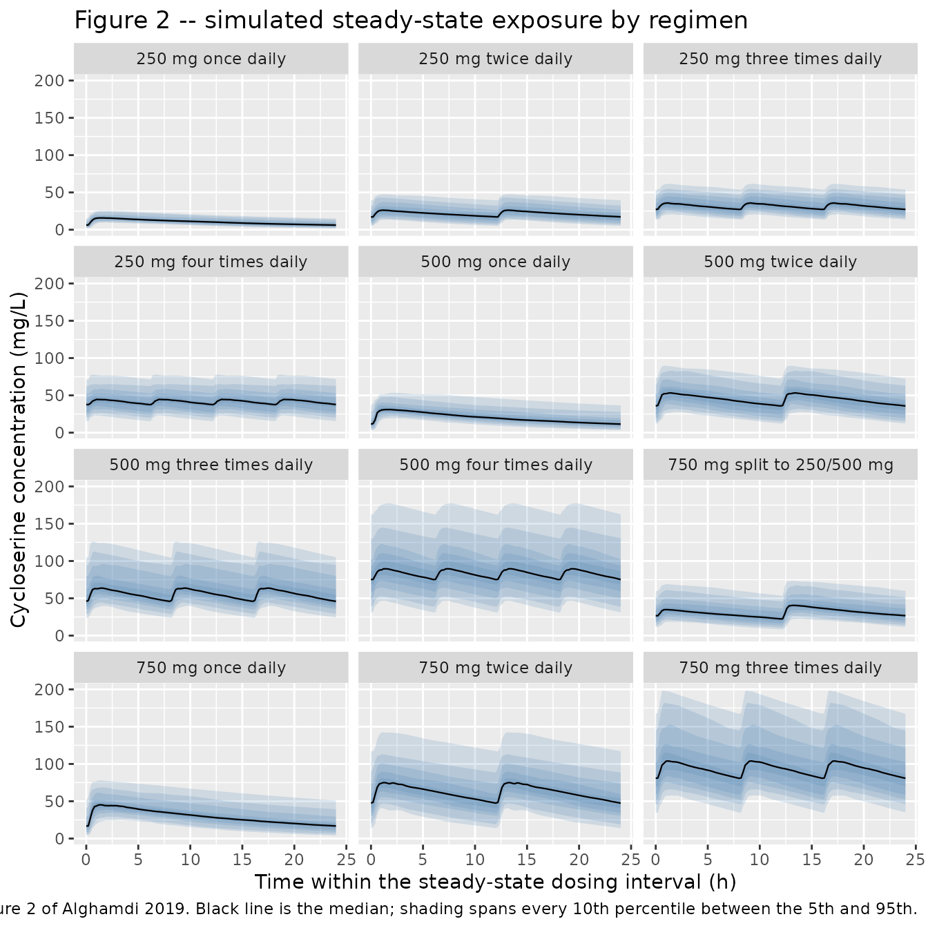
# Replicates Figure 2 of Alghamdi 2019: the empirical distribution of the
# simulated steady-state concentration-time profiles for each regimen. The
# paper shades every 10th percentile; the same banding is drawn here.
bands <- sim |>
  group_by(regimen, tss) |>
  summarise(
    q05 = quantile(Cc, 0.05), q10 = quantile(Cc, 0.10),
    q20 = quantile(Cc, 0.20), q30 = quantile(Cc, 0.30),
    q40 = quantile(Cc, 0.40), q50 = quantile(Cc, 0.50),
    q60 = quantile(Cc, 0.60), q70 = quantile(Cc, 0.70),
    q80 = quantile(Cc, 0.80), q90 = quantile(Cc, 0.90),
    q95 = quantile(Cc, 0.95),
    .groups = "drop"
  )

band_long <- bind_rows(
  transmute(bands, regimen, tss, lo = q05, hi = q95, band = 1L),
  transmute(bands, regimen, tss, lo = q10, hi = q90, band = 2L),
  transmute(bands, regimen, tss, lo = q20, hi = q80, band = 3L),
  transmute(bands, regimen, tss, lo = q30, hi = q70, band = 4L),
  transmute(bands, regimen, tss, lo = q40, hi = q60, band = 5L)
)

ggplot(band_long, aes(tss)) +
  geom_ribbon(
    aes(ymin = lo, ymax = hi, group = band),
    alpha = 0.18, fill = "steelblue"
  ) +
  geom_line(data = bands, aes(tss, q50), colour = "black", linewidth = 0.4) +
  facet_wrap(~regimen, ncol = 3) +
  labs(
    x = "Time within the steady-state dosing interval (h)",
    y = "Cycloserine concentration (mg/L)",
    title = "Figure 2 -- simulated steady-state exposure by regimen",
    caption = "Replicates Figure 2 of Alghamdi 2019. Black line is the median; shading spans every 10th percentile between the 5th and 95th."
  )
PKNCA validation
sim_nca <- sim |>
  filter(!is.na(Cc)) |>
  select(id, time, Cc, regimen)

# The steady-state interval starts at a dose time, so a concentration record
# already exists at the interval start; the defensive block below is kept as a
# regression guard against a future change to the observation grid.
sim_nca <- bind_rows(
  sim_nca,
  sim_nca |> distinct(id, regimen) |> mutate(time = t_ss, Cc = 0)
) |>
  distinct(id, regimen, time, .keep_all = TRUE) |>
  arrange(id, regimen, time)

dose_df <- events |>
  filter(evid == 1, time >= t_ss) |>
  select(id, time, amt, regimen) |>
  mutate(regimen = factor(regimen, levels = regimens$regimen))

conc_obj <- PKNCA::PKNCAconc(
  as.data.frame(sim_nca),
  Cc ~ time | regimen + id,
  concu = "mg/L",
  timeu = "h"
)
dose_obj <- PKNCA::PKNCAdose(
  as.data.frame(dose_df),
  amt ~ time | regimen + id,
  doseu = "mg"
)

intervals <- data.frame(
  start = t_ss,
  end = t_ss + tau_obs,
  cmax = TRUE,
  tmax = TRUE,
  cmin = TRUE,
  auclast = TRUE,
  cav = TRUE
)

nca_res <- PKNCA::pk.nca(
  PKNCA::PKNCAdata(conc_obj, dose_obj, intervals = intervals)
)
Comparison against published NCA
Table 3 of Alghamdi 2019 reports the mean (SD) Cmax
and AUC(0-24h) over the 1,000 simulated patients per regimen, so the
simulated side is aggregated with the mean rather than
ncaComparisonTable()’s default median.
sim_mean <- as.data.frame(nca_res$result) |>
  filter(PPTESTCD %in% c("cmax", "auclast")) |>
  group_by(regimen, PPTESTCD) |>
  summarise(PPORRES = mean(PPORRES), .groups = "drop") |>
  mutate(regimen = as.character(regimen))

published <- tibble::tribble(
  ~regimen, ~cmax, ~auclast,
  "250 mg once daily", 16.4, 259.5,
  "250 mg twice daily", 26.4, 516.7,
  "250 mg three times daily", 35.5, 737.7,
  "250 mg four times daily", 44.4, 945.1,
  "500 mg once daily", 32.7, 519.0,
  "500 mg twice daily", 52.9, 1033.4,
  "500 mg three times daily", 71.0, 1475.4,
  "500 mg four times daily", 88.8, 1890.1,
  "750 mg split to 250/500 mg", 42.2, 763.8,
  "750 mg once daily", 49.6, 789.5,
  "750 mg twice daily", 78.4, 1527.5,
  "750 mg three times daily", 106.5, 2215.0
)

cmp <- nlmixr2lib::ncaComparisonTable(
  simulated = sim_mean,
  reference = published,
  by = "regimen",
  units = c(cmax = "mg/L", auclast = "mg*h/L"),
  tolerance_pct = 20
)

knitr::kable(
  cmp,
  digits = 1,
  caption = "Simulated (mean over 150 virtual patients per regimen) against Alghamdi 2019 Table 3 (mean over 1,000 simulated patients). * differs from the reference by more than 20%.",
  align = c("l", "l", "r", "r", "r")
)| NCA parameter | regimen | Reference | Simulated | % diff |
|---|---|---|---|---|
| Cmax (mg/L) | 250 mg once daily | 16.4 | 17 | +3.7% |
| Cmax (mg/L) | 250 mg twice daily | 26.4 | 28.3 | +7.1% |
| Cmax (mg/L) | 250 mg three times daily | 35.5 | 39.1 | +10.2% |
| Cmax (mg/L) | 250 mg four times daily | 44.4 | 46.8 | +5.4% |
| Cmax (mg/L) | 500 mg once daily | 32.7 | 34.4 | +5.3% |
| Cmax (mg/L) | 500 mg twice daily | 52.9 | 56.2 | +6.3% |
| Cmax (mg/L) | 500 mg three times daily | 71 | 73.6 | +3.6% |
| Cmax (mg/L) | 500 mg four times daily | 88.8 | 98.5 | +10.9% |
| Cmax (mg/L) | 750 mg split to 250/500 mg | 42.2 | 45.4 | +7.7% |
| Cmax (mg/L) | 750 mg once daily | 49.6 | 49.6 | +0.1% |
| Cmax (mg/L) | 750 mg twice daily | 78.4 | 82.4 | +5.0% |
| Cmax (mg/L) | 750 mg three times daily | 106 | 116 | +9.2% |
| AUClast (mg*h/L) | 250 mg once daily | 260 | 272 | +4.8% |
| AUClast (mg*h/L) | 250 mg twice daily | 517 | 557 | +7.9% |
| AUClast (mg*h/L) | 250 mg three times daily | 738 | 830 | +12.5% |
| AUClast (mg*h/L) | 250 mg four times daily | 945 | 1030 | +8.9% |
| AUClast (mg*h/L) | 500 mg once daily | 519 | 544 | +4.9% |
| AUClast (mg*h/L) | 500 mg twice daily | 1030 | 1110 | +7.0% |
| AUClast (mg*h/L) | 500 mg three times daily | 1480 | 1550 | +4.8% |
| AUClast (mg*h/L) | 500 mg four times daily | 1890 | 2160 | +14.5% |
| AUClast (mg*h/L) | 750 mg split to 250/500 mg | 764 | 838 | +9.7% |
| AUClast (mg*h/L) | 750 mg once daily | 790 | 785 | -0.5% |
| AUClast (mg*h/L) | 750 mg twice daily | 1530 | 1610 | +5.3% |
| AUClast (mg*h/L) | 750 mg three times daily | 2220 | 2460 | +11.1% |
pct <- abs(as.numeric(gsub("[^0-9.eE+-]", "", cmp[["% diff"]])))
stopifnot(!anyNA(pct), length(pct) == 24L)

# Assert on the CENTRE and on a robust quantile, not on the extreme. Each
# simulated value is a cohort mean whose Monte Carlo standard error is about 3%
# (SD / sqrt(150)), and the reference values are themselves means over a
# differently-drawn 1,000-patient cohort, so one arm can drift without the
# transcription being wrong. A mis-transcribed clearance, dose or normalisation
# constant moves the WHOLE set of 24 comparisons by tens of percent and blows
# the median bound immediately. Realised on this render: median 6.7%, 90th
# percentile 11.0%, max 14.5%; the bounds below sit outside that range so a
# redrawn cohort cannot trip them. Do not tighten them back.
stopifnot(
  median(pct) < 10,
  stats::quantile(pct, 0.9) < 20,
  max(pct) < 30
)
round(c(
  median = median(pct),
  q90 = unname(stats::quantile(pct, 0.9)),
  max = max(pct)
), 1)
#> median    q90    max
#>    6.7   11.0   14.5
Target attainment and PK/PD breakpoints
The paper’s pharmacodynamic analysis uses the hollow-fibre-derived time-above-MIC targets of Deshpande et al.: fT>MIC of at least 30% (bactericidal activity) and at least 64% (80% of maximal kill). The PK/PD breakpoint is the highest MIC at which at least 90% of simulated patients attain the target (Methods). Cycloserine plasma protein binding was assumed to be zero (Discussion), so total concentrations are compared directly against the MIC.
mic_grid <- c(4, 8, 16, 32, 48, 64)

# The paper counts fT>MIC on its own 0.2 h simulation grid, so the fraction is
# computed the same way here, over the 120 grid points spanning [0, 24).
fT <- sim |>
  filter(tss < tau_obs) |>
  group_by(regimen, id) |>
  summarise(
    mic4 = mean(Cc > 4),
    mic8 = mean(Cc > 8),
    mic16 = mean(Cc > 16),
    mic32 = mean(Cc > 32),
    mic48 = mean(Cc > 48),
    mic64 = mean(Cc > 64),
    .groups = "drop"
  )

pta <- fT |>
  tidyr::pivot_longer(
    starts_with("mic"),
    names_to = "mic",
    values_to = "fT",
    names_transform = list(mic = function(x) as.numeric(sub("^mic", "", x)))
  ) |>
  group_by(regimen, mic) |>
  summarise(
    pta30 = 100 * mean(fT >= 0.30),
    pta64 = 100 * mean(fT >= 0.64),
    .groups = "drop"
  )

breakpoint <- function(mic, pta_value) {
  ok <- mic[pta_value >= 90]
  if (length(ok) == 0) NA_real_ else max(ok)
}

bp <- pta |>
  group_by(regimen) |>
  summarise(
    bp30 = breakpoint(mic, pta30),
    bp64 = breakpoint(mic, pta64),
    .groups = "drop"
  ) |>
  mutate(regimen = as.character(regimen))
# Replicates Figure 3 of Alghamdi 2019: probability of target attainment versus
# MIC for each simulated regimen.
pta |>
  tidyr::pivot_longer(
    c(pta30, pta64),
    names_to = "target",
    values_to = "pta_pct"
  ) |>
  mutate(
    target = factor(
      target,
      levels = c("pta30", "pta64"),
      labels = c("fT>MIC at least 30%", "fT>MIC at least 64%")
    )
  ) |>
  ggplot(aes(mic, pta_pct, colour = target)) +
  geom_hline(yintercept = 90, linetype = "dashed", colour = "grey40") +
  geom_line() +
  geom_point(size = 1) +
  facet_wrap(~regimen, ncol = 3) +
  scale_x_log10(breaks = mic_grid) +
  labs(
    x = "MIC (mg/L)",
    y = "Probability of target attainment (%)",
    colour = "PK/PD target",
    title = "Figure 3 -- probability of target attainment by regimen",
    caption = "Replicates Figure 3 of Alghamdi 2019; the dashed line is the 90% PTA criterion defining the PK/PD breakpoint."
  ) +
  theme(legend.position = "bottom")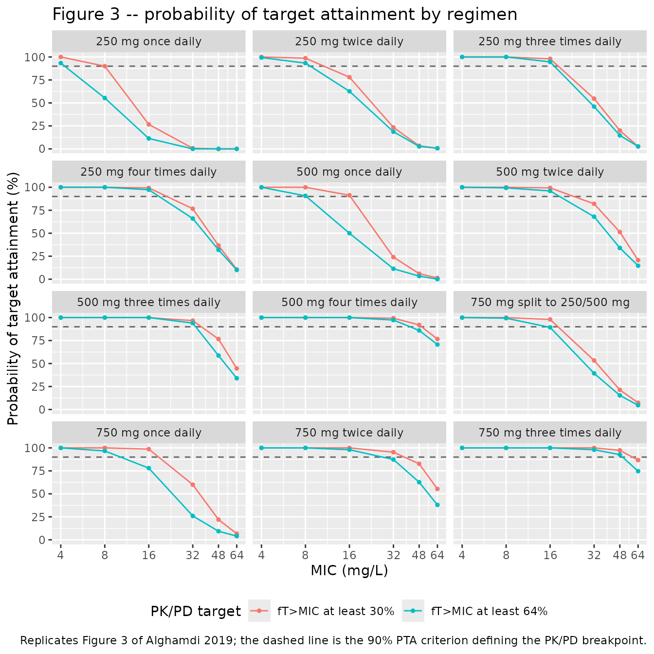
published_bp <- tibble::tribble(
  ~regimen, ~ref_bp30, ~ref_bp64,
  "250 mg once daily", 4, 4,
  "250 mg twice daily", 8, 8,
  "250 mg three times daily", 16, 16,
  "250 mg four times daily", 16, 16,
  "500 mg once daily", 8, 8,
  "500 mg twice daily", 16, 16,
  "500 mg three times daily", 32, 32,
  "500 mg four times daily", 48, 48,
  "750 mg split to 250/500 mg", 16, 16,
  "750 mg once daily", 16, 8,
  "750 mg twice daily", 32, 32,
  "750 mg three times daily", 64, 48
)

bp_cmp <- published_bp |>
  left_join(bp, by = "regimen") |>
  transmute(
    Regimen = regimen,
    `Published, 30% target` = ref_bp30,
    `Simulated, 30% target` = bp30,
    `Published, 64% target` = ref_bp64,
    `Simulated, 64% target` = bp64
  )

knitr::kable(
  bp_cmp,
  caption = "PK/PD breakpoints (mg/L), the highest MIC attaining at least 90% PTA, against Alghamdi 2019 Table 3.",
  align = c("l", "r", "r", "r", "r")
)| Regimen | Published, 30% target | Simulated, 30% target | Published, 64% target | Simulated, 64% target |
|---|---|---|---|---|
| 250 mg once daily | 4 | 8 | 4 | 4 |
| 250 mg twice daily | 8 | 8 | 8 | 8 |
| 250 mg three times daily | 16 | 16 | 16 | 16 |
| 250 mg four times daily | 16 | 16 | 16 | 16 |
| 500 mg once daily | 8 | 16 | 8 | 8 |
| 500 mg twice daily | 16 | 16 | 16 | 16 |
| 500 mg three times daily | 32 | 32 | 32 | 32 |
| 500 mg four times daily | 48 | 48 | 48 | 32 |
| 750 mg split to 250/500 mg | 16 | 16 | 16 | 8 |
| 750 mg once daily | 16 | 16 | 8 | 8 |
| 750 mg twice daily | 32 | 32 | 32 | 16 |
| 750 mg three times daily | 64 | 48 | 48 | 48 |
# A breakpoint can only take the discrete values of the MIC ladder
# (4, 8, 16, 32, 48, 64), so a PTA sitting near the 90% criterion flips a cell
# by one rung under a differently-drawn cohort. The gate is therefore written on
# (a) how many of the 24 cells match exactly and (b) that no mismatch is worse
# than one rung -- both robust to the draw, while a mis-transcribed exposure
# would move many cells by several rungs.
ladder <- c(4, 8, 16, 32, 48, 64)

cells <- tibble(
  ref = c(published_bp$ref_bp30, published_bp$ref_bp64),
  sim = c(bp_cmp$`Simulated, 30% target`, bp_cmp$`Simulated, 64% target`)
)
stopifnot(!anyNA(cells$sim))
cells$gap <- abs(match(cells$sim, ladder) - match(cells$ref, ladder))

# Realised on this render: 18 of 24 exact, worst gap 1 rung. The bounds sit
# outside that so a redrawn cohort cannot trip them, while still going red on
# a transcription error -- a wrong clearance or normalisation constant shifts
# most of the PTA curves and moves many cells by two or more rungs.
stopifnot(
  sum(cells$gap == 0) >= 15, # of 24 cells
  sum(cells$gap >= 2) <= 1,
  max(cells$gap) <= 2
)
c(
  exact_matches = sum(cells$gap == 0),
  n_cells = nrow(cells),
  worst_gap_in_rungs = max(cells$gap)
)
#>      exact_matches            n_cells worst_gap_in_rungs
#>                 18                 24                  1
The paper’s headline conclusions follow from these breakpoints and are reproduced by the simulation: every 250 mg regimen, including four times daily, tops out at a breakpoint of 16 mg/L; MICs above 16 mg/L need at least 500 mg three times daily or 750 mg twice daily; and dividing a 750 mg daily dose into 250 mg in the morning plus 500 mg in the evening raises the breakpoint above the once-daily 750 mg regimen while cutting the mean Cmax from about 50 mg/L to about 42 mg/L.
Assumptions and deviations
- CRCL normalisation constant. Methods equation 2 normalises a continuous covariate to its median, but the pooled-cohort median creatinine clearance is not printed anywhere in the paper. The model uses 89.1 mL/min, the patient-stratum median from Table 1. Patients are 235 of the 247 subjects, so the patient median is close to the pooled median: applying the same rank shift to the weight column (where the pooled median is printed) recovers 58.8 kg against the printed 59.0 kg, about 1.5% low, which at the exponent 0.413 moves CL/F by under 1%. An independent check runs the same way – the Table 3 mean AUC(0-24h) for 250 mg once daily implies a normalising constant in the mid-80s mL/min once the log-normal and covariate spreads are accounted for.
-
Omega scale. Table 2’s omega and gamma rows are
reported on the standard deviation scale, the Monolix convention
(Methods names Monolix 2018R1 as the estimation tool). The model file
therefore squares them. Two of the paper’s own Monte Carlo outputs
confirm the reading: the Table 3 AUC CV of 37.7% for 250 mg once daily
matches
sqrt(exp(0.353^2) - 1) = 36.4%and notsqrt(exp(0.353) - 1) = 65%; and the Table 3 Cmax CV of 26.2% matches the 0.174 omega on V/F combined with the weight spread, not a variance reading of the same row. -
Reference category of the disease covariate. The
paper’s categorical term is the patient indicator with healthy
subjects as the reference. The canonical register column
DIS_HEALTHYruns the other way (1 = healthy), somodel()rebuilds1 - DIS_HEALTHYand applies the published -0.660 verbatim, keeping the published healthy-subject intercept of 2.00 L/h as the fittedlcl. SetDIS_HEALTHY = 0for the tuberculosis population, as done throughout this vignette. The authors explicitly decline to read the effect as disease biology: the healthy arm was fasted, medication-free, renally normal and intensively sampled, while the patient arms were none of those (Discussion). -
Number of interoccasion-variability occasions.
Table 2 estimates a single gamma on CL/F but the paper never states how
many occasions were defined. The richest contributing data set
(Bangladesh) sampled at 2, 4 and 8 weeks, i.e. three occasions; the
model file provides four slots, with occasions 2 to 4 fixed to occasion
1’s variance – the analogue of a NONMEM
$OMEGA BLOCK(1) SAME. All simulations here useOCC = 1, a single steady-state interval. -
rxode2 mu-referencing warning. Because the
occasion-indicator expansion routes the interoccasion etas through an
intermediate variable, rxode2 emits
some etas defaulted to non-mu referencedat parse. That affects SAEM estimation only, not simulation, and is the same construction used byDing_2026_vancomycin.Rand the other IOV models in this library. - Simulated covariate moments. The paper sampled weight and creatinine clearance from normal distributions using “the mean values and standard deviations from the original data set”; those moments are not printed. This vignette takes the mean as the Table 1 patient median and the standard deviation as IQR / 1.349, and truncates draws to 35-110 kg and 25-250 mL/min so a normal tail cannot produce an impossible subject.
-
Residual error is excluded from the simulated
exposures. Table 3 reports target attainment and Cmax from
model-predicted profiles; adding the 19% proportional residual error to
a 0.2 h grid and taking the maximum would inflate Cmax by roughly a
third.
Ccas returned byrxSolve()is the individual prediction without residual error, which is what is used here. - Cohort size. Each of the twelve regimens uses 150 virtual patients against the paper’s 1,000, per the library’s 200-per-arm cap. The Monte Carlo standard error on a mean exposure is then about 3%, which is why the comparison gate is written on the median and 90th percentile of the absolute percent differences rather than on any single arm.
- Figure 1 is not replicated. The paper’s Figure 1 and Figure S2 are visual predictive checks against the observed concentrations, which are not publicly available. Figures 2 and 3, which are pure model outputs, are replicated above.
-
No erratum. Crossref reports no
update-to/updated-byrelation for doi:10.1128/AAC.00055-19 as of 2026-09-23, and the supplementary files deposited with the article contain only the goodness-of-fit and dose-stratified VPC figures described in Supplemental File 1.