Letermovir (Royston 2025)
Source:vignettes/articles/Royston_2025_letermovir.Rmd
Royston_2025_letermovir.RmdModel and source
- Citation: Royston L, Kunz C, Tonoli D, Lescuyer P, Neofytos D, Gotta V (2025). Population pharmacokinetic analysis of letermovir in adult hematopoietic cell transplant recipients. Antimicrob Agents Chemother 69(10):e00697-25. doi:10.1128/aac.00697-25. Ka, Tlag and the IIV on Ka and V/F were fixed from the phase III model of Prohn et al. (2021) CPT Pharmacometrics Syst Pharmacol 10:255-267, doi:10.1002/psp4.12593, as reproduced in Royston 2025 Table 1.
- Description: One-compartment population PK model with first-order absorption and absorption lag time for oral letermovir in adult allogeneic hematopoietic cell transplant recipients, with a cyclosporine effect on apparent oral clearance and inter-occasion variability on CL/F
- Article: https://doi.org/10.1128/aac.00697-25
- Upstream phase III model (source of the fixed Ka, Tlag and their IIV): Prohn et al. (2021) https://doi.org/10.1002/psp4.12593
Royston 2025 is a short-form post hoc pharmacometric analysis of a prospective therapeutic drug monitoring study in allogeneic hematopoietic cell transplant (HCT) recipients receiving oral letermovir as primary cytomegalovirus prophylaxis. The paper makes two claims: (1) the industry-sponsored phase III model of Prohn 2021 substantially over-predicts real-world letermovir concentrations, and (2) a simplified one-compartment model refitted to the real-world data describes them much better (AIC 4,830 -> 3,739).
This vignette packages and validates the adjusted real-world model – the model the authors themselves fitted, reported in the right-hand column of Table 1. The phase III comparator model is not packaged here; see Assumptions and deviations for why.
Population
pop <- rxode2::rxode(readModelDb("Royston_2025_letermovir"))$population
#> ℹ parameter labels from comments will be replaced by 'label()'
#> Warning: some etas defaulted to non-mu referenced, possible parsing error: etaiov_cl_1, etaiov_cl_2, etaiov_cl_3, etaiov_cl_4, etaiov_cl_5, etaiov_cl_6, etaiov_cl_7, etaiov_cl_8
#> as a work-around try putting the mu-referenced expression on a simple line
str(pop)
#> List of 7
#>  $ species      : chr "human"
#>  $ n_subjects   : num 40
#>  $ n_studies    : num 1
#>  $ disease_state: chr "adult CMV-seropositive allogeneic hematopoietic cell transplant recipients receiving primary CMV prophylaxis"
#>  $ dose_range   : chr "480 mg orally once daily, or 240 mg orally once daily when coadministered with cyclosporine"
#>  $ regions      : chr "Switzerland (University Hospitals of Geneva)"
#>  $ notes        : chr "Post hoc pharmacometric analysis of a prospective observational therapeutic drug monitoring study conducted bet"| __truncated__
Forty adult CMV-seropositive allogeneic HCT recipients received primary CMV prophylaxis with oral letermovir between 1 March 2020 and 20 April 2021 at the University Hospitals of Geneva, dosed once daily at 480 mg, or at 240 mg when coadministered with cyclosporine (6 of the 40 patients). The analysis pooled 296 plasma concentrations: 217 trough samples drawn 24 +/- 2 h post-dose and 79 non-trough samples.
This short-form publication does not tabulate baseline demographics; age, weight and sex distributions are reported in the parent study (Royston 2022, https://doi.org/10.1128/aac.00657-22). Because the final model in Table 1 carries no demographic covariates, the absence of those distributions does not affect the simulations below.
Source trace
Every ini() entry in
inst/modeldb/specificDrugs/Royston_2025_letermovir.R
carries an in-file comment naming its origin. They are collected here
for review. All values come from the “Adjusted model estimate
from one-compartmental model fitted to real-world data” column
of Royston 2025 Table 1 unless noted.
| Equation / parameter | Value | Source location |
|---|---|---|
lka (fixed) |
log(0.15) 1/h |
Table 1, Ka row: “0.15 (fixed)” – fixed from the Prohn 2021 phase III model |
ltlag (fixed) |
log(0.674) h |
Table 1, Tlag row: “0.674 (fixed)” – fixed from Prohn 2021 |
lcl |
log(26.5) L/h |
Table 1, CL/F row: 26.5 (RSE 12.6%) |
lvc |
log(115.2) L |
Table 1, V/F row: 115.2 (RSE 12%) |
e_csa_cl |
-0.38 |
Table 1, fCSA row: -0.38 (RSE 69.5%) |
etalka (fixed) |
0.72^2 |
Table 1, Ka row [0.72 (fixed)]; footnote a: SD of
log-transformed parameter |
etalvc (fixed) |
0.23^2 |
Table 1, V/F row [0.23 (fixed)]; footnote a |
etalcl |
0.58^2 |
Table 1, CL/F row [IIV 0.58 (RSE 17%)]; footnote a |
etaiov_cl_1..8 |
0.62^2 |
Table 1, CL/F row [IOV 0.62 (RSE 7%)]; footnote a |
propSd |
0.29 |
Table 1, “Residual error (%/ug/L)” row: “29%/-” (proportional only, no additive term) |
d/dt(depot), d/dt(central),
alag(depot)
|
n/a | Results: “simplified one-compartment with fixed absorption rate and lag time”; Discussion: “Simplifications to an oral one-compartment model appear justified given the lack of bi-phasic decline during 24-h dosing intervals (Fig. 1)” |
cl <- ... * exp(e_csa_cl * CONMED_CSA) |
n/a | Results: CL/F “reduced by 32% with cyclosporin”; see the falsifier note below |
Why the cyclosporine effect is exponential, not linear
Table 1 reports fCSA = -0.38, but the Results text
states that CL/F is “reduced by 32% with cyclosporin”. Those
two numbers pin the functional form exactly:
1 - exp(-0.38) is 31.6%, which rounds to the quoted 32%;
a linear 1 - 0.38 form would have been quoted as 38%. The
multiplicative-on-log-scale form is therefore the one the authors
fitted, and it is also Monolix’s standard parameterization for a
categorical covariate on a log-normally distributed parameter. (The
Discussion separately restates the raw coefficient as “-38%”, which is
the coefficient value, not the back-transformed effect.)
Virtual cohort
Original observed data are not publicly available. Two arms of 200 virtual subjects each reproduce the study’s two regimens. The final model carries no demographic covariates, so the only subject-level inputs are the cyclosporine indicator and the occasion index.
Each subject receives 8 consecutive once-daily doses, one per
occasion (OCC = 1..8), matching the paper’s treatment of
each patient visit as a separate occasion. A trough sample is drawn at
the end of every dosing interval, and the final interval is additionally
sampled densely for NCA.
Note that the sample at time = 168 h serves twice over:
it is occasion 7’s end-of-interval trough and, because the
0.674 h absorption lag leaves the concentration continuous across a
dose, it is also occasion 8’s time-zero concentration. Everything
downstream is therefore keyed off time rather than off a
recomputed occasion index, which would have to classify that row as one
or the other.
set.seed(20250822)

n_per_arm <- 200L
n_occ <- 8L
tau <- 24
t_last <- tau * (n_occ - 1L)  # dose time opening the final interval

make_arm <- function(n, dose, csa, label, id_offset = 0L) {
  ids <- id_offset + seq_len(n)

  doses <- tidyr::expand_grid(id = ids, time = tau * (seq_len(n_occ) - 1L)) |>
    dplyr::mutate(
      amt = dose, evid = 1L, cmt = "depot",
      OCC = as.integer(time / tau) + 1L
    )

  # Trough samples: end of every dosing interval. The sample ending occasion k
  # coincides with the dose opening occasion k+1; sorting evid = 0 ahead of
  # evid = 1 makes it a pre-dose sample, which is what the paper drew. The
  # covariate OCC on that row is k, so it is eliminated under occasion k's CL/F.
  troughs <- tidyr::expand_grid(id = ids, time = tau * seq_len(n_occ)) |>
    dplyr::mutate(OCC = as.integer(time / tau))

  # Dense grid over the final dosing interval only, for NCA and the profile.
  dense <- tidyr::expand_grid(id = ids, time = seq(t_last, tau * n_occ, by = 0.5)) |>
    dplyr::mutate(OCC = n_occ)

  obs <- dplyr::bind_rows(troughs, dense) |>
    dplyr::distinct(id, time, .keep_all = TRUE) |>
    dplyr::mutate(amt = NA_real_, evid = 0L, cmt = "central")

  dplyr::bind_rows(doses, obs) |>
    dplyr::mutate(CONMED_CSA = csa, treatment = label, dose_mg = dose) |>
    dplyr::arrange(id, time, evid)
}

events <- dplyr::bind_rows(
  make_arm(n_per_arm, 480, 0L, "480 mg QD", id_offset = 0L),
  make_arm(n_per_arm, 240, 1L, "240 mg QD + CSA", id_offset = n_per_arm)
)

stopifnot(!anyDuplicated(events[, c("id", "time", "evid")]))
stopifnot(length(unique(events$id)) == 2L * n_per_arm)
Simulation
mod <- readModelDb("Royston_2025_letermovir")

sim <- rxode2::rxSolve(
  mod,
  events = events,
  keep = c("treatment", "CONMED_CSA", "OCC", "dose_mg"),
  addDosing = FALSE,
  # The occasion-k trough and the occasion-(k+1) dose share a time stamp, and
  # rxode2 orders the dose row first internally, so under the default
  # last-observation-carried-forward interpolation the ODE integrator carries
  # occasion k's OCC -- and so its CL/F -- into the first step of occasion
  # k+1 (measured: 0.38% median / 9% max error in the mass balance below).
  # Next-observation-carried-backward, the NONMEM convention, applies each
  # row's OCC to the interval that ends at that row, which is the design
  # described above and what the analytic solution does.
  covsInterpolation = "nocb"
) |>
  as.data.frame() |>
  dplyr::mutate(
    is_trough = time > 0 & abs(time %% tau) < 1e-8,
    in_last = time >= t_last,
    tad_last = time - t_last
  )
#> ℹ parameter labels from comments will be replaced by 'label()'
#> Warning: some etas defaulted to non-mu referenced, possible parsing error: etaiov_cl_1, etaiov_cl_2, etaiov_cl_3, etaiov_cl_4, etaiov_cl_5, etaiov_cl_6, etaiov_cl_7, etaiov_cl_8
#> as a work-around try putting the mu-referenced expression on a simple line

stopifnot(nrow(sim) > 0, !anyNA(sim$Cc), all(sim$Cc >= 0))
# Every subject must contribute one trough per occasion.
stopifnot(all(table(sim$id[sim$is_trough]) == n_occ))
Cc is the individual prediction and carries no residual
error; the sim column adds the 29% proportional residual
error. Comparisons against observed concentrations below use
sim, because the published troughs are measured values that
include assay error. Structural checks use Cc.
A typical-value companion simulation, with every random effect zeroed, is used below for the deterministic checks.
mod_typical <- rxode2::zeroRe(rxode2::rxode(mod))
#> ℹ parameter labels from comments will be replaced by 'label()'
#> Warning: some etas defaulted to non-mu referenced, possible parsing error: etaiov_cl_1, etaiov_cl_2, etaiov_cl_3, etaiov_cl_4, etaiov_cl_5, etaiov_cl_6, etaiov_cl_7, etaiov_cl_8
#> as a work-around try putting the mu-referenced expression on a simple line
#> Warning: some etas defaulted to non-mu referenced, possible parsing error: etaiov_cl_1, etaiov_cl_2, etaiov_cl_3, etaiov_cl_4, etaiov_cl_5, etaiov_cl_6, etaiov_cl_7, etaiov_cl_8
#> as a work-around try putting the mu-referenced expression on a simple line

sim_typ <- rxode2::rxSolve(
  mod_typical,
  events |> dplyr::filter(id %in% c(1L, 1L + n_per_arm)),
  keep = c("treatment", "dose_mg"), addDosing = FALSE
) |>
  as.data.frame() |>
  dplyr::mutate(is_trough = time > 0 & abs(time %% tau) < 1e-8,
                in_last = time >= t_last,
                tad_last = time - t_last)
#> ℹ omega/sigma items treated as zero: 'etalcl', 'etalka', 'etalvc', 'etaiov_cl_1', 'etaiov_cl_2', 'etaiov_cl_3', 'etaiov_cl_4', 'etaiov_cl_5', 'etaiov_cl_6', 'etaiov_cl_7', 'etaiov_cl_8'
#> Warning: multi-subject simulation without without 'omega'
Steady state
At the typical value the model is flip-flop: ka (0.15
1/h, half-life 4.6 h) is slower than kel (CL/F divided by
V/F, 0.23 1/h), so the terminal phase is absorption-limited with a 4.6 h
half-life against a 24 h dosing interval. Accumulation is
correspondingly slight, which is what makes the paper’s treatment of
“each patient visit as an occasion at steady state” reasonable.
typ_accum <- sim_typ |>
  dplyr::filter(is_trough) |>
  dplyr::mutate(occ = as.integer(time / tau)) |>
  dplyr::select(treatment, occ, Cc) |>
  dplyr::mutate(trough_ng_mL = 1000 * Cc) |>
  dplyr::select(-Cc) |>
  tidyr::pivot_wider(names_from = occ, values_from = trough_ng_mL)

knitr::kable(typ_accum, digits = 1,
caption = "Typical-value trough by occasion (ng/mL).")| treatment | 1 | 2 | 3 | 4 | 5 | 6 | 7 | 8 |
|---|---|---|---|---|---|---|---|---|
| 480 mg QD | 199.6 | 205.9 | 206.1 | 206.1 | 206.1 | 206.1 | 206.1 | 206.1 |
| 240 mg QD + CSA | 202.6 | 212.9 | 213.3 | 213.3 | 213.3 | 213.3 | 213.3 | 213.3 |
# Accumulation, and confirmation that the plateau is genuinely reached.
typ_ratio <- sim_typ |>
  dplyr::filter(is_trough) |>
  dplyr::group_by(treatment) |>
  dplyr::summarise(
    accumulation_occ8_over_occ1 = Cc[time == tau * n_occ] / Cc[time == tau],
    plateau_occ8_over_occ4 = Cc[time == tau * n_occ] / Cc[time == tau * 4],
    .groups = "drop"
  )
knitr::kable(typ_ratio, digits = 5,
caption = "Typical-value accumulation and plateau ratios.")| treatment | accumulation_occ8_over_occ1 | plateau_occ8_over_occ4 |
|---|---|---|
| 240 mg QD + CSA | 1.05297 | 1 |
| 480 mg QD | 1.03249 | 1 |
# A single-exponential approximation using the absorption-limited terminal rate.
# It under-states the 240 mg + CSA arm because there kel (0.157) sits very close
# to ka (0.15), so the second exponential still contributes at trough.
c(single_exponential_approximation = 1 / (1 - exp(-0.15 * tau)))
#> single_exponential_approximation
#>                         1.028091

# Total accumulation over eight occasions is under 6% in both arms ...
stopifnot(all(typ_ratio$accumulation_occ8_over_occ1 > 1.02),
          all(typ_ratio$accumulation_occ8_over_occ1 < 1.06))
# ... and the trough is flat to within 0.1% from occasion 4 onward, so the
# final interval is unambiguously at steady state.
stopifnot(all(abs(typ_ratio$plateau_occ8_over_occ4 - 1) < 1e-3))
That tidy picture holds only near the centre of the population. IIV
on CL/F and V/F, plus an inter-occasion SD of 0.62 on CL/F, spread
kel widely, and subjects in the low-clearance tail have
kel < ka and accumulate materially across occasions. The
paper’s per-occasion steady-state approximation is therefore good for a
typical patient and progressively weaker in that tail – worth knowing
before reusing this model for an accumulation question.
Replicate published figures
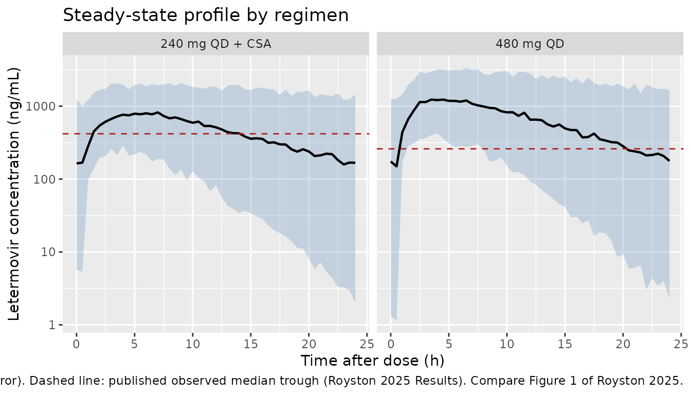
# Replicates Figure 1 of Royston 2025: letermovir concentrations on a
# time-after-dose scale, by regimen. Royston 2025 plots the real-world
# observations against the phase III model's expected profile; here the ribbon
# is the adjusted (real-world) model's own prediction interval, and the dashed
# line marks the published observed median trough for each regimen.
published_trough <- tibble::tribble(
  ~treatment,         ~median, ~q1,  ~q3,
  "480 mg QD",         260,     123,  518,
  "240 mg QD + CSA",   418,     235,  945
)

sim |>
  dplyr::filter(in_last) |>
  dplyr::group_by(treatment, tad_last) |>
  dplyr::summarise(
    Q05 = 1000 * quantile(sim, 0.05),
    Q50 = 1000 * quantile(sim, 0.50),
    Q95 = 1000 * quantile(sim, 0.95),
    .groups = "drop"
  ) |>
  ggplot(aes(tad_last, Q50)) +
  geom_ribbon(aes(ymin = Q05, ymax = Q95), alpha = 0.25, fill = "steelblue") +
  geom_line(linewidth = 0.8) +
  geom_hline(
    data = published_trough,
    aes(yintercept = median), linetype = "dashed", colour = "firebrick"
  ) +
  facet_wrap(~treatment) +
  scale_y_log10() +
  labs(
    x = "Time after dose (h)", y = "Letermovir concentration (ng/mL)",
    title = "Steady-state profile by regimen",
    caption = paste(
      "Adjusted-model prediction interval (5th-50th-95th percentile, with",
      "residual error). Dashed line: published observed median trough",
      "(Royston 2025 Results). Compare Figure 1 of Royston 2025."
    )
  )
PKNCA validation
NCA runs on the final dosing interval, rebased so time 0 is the dose
opening that interval. The time = 168 h sample supplies the
time-zero concentration directly, so no zero is imputed.
nca_conc <- sim |>
  dplyr::filter(in_last, !is.na(Cc)) |>
  dplyr::select(id, time = tad_last, Cc, treatment) |>
  dplyr::arrange(id, treatment, time)

# A real time-zero record must already be present (steady-state pre-dose
# concentration), not an imputed zero.
stopifnot(all(tapply(nca_conc$time, nca_conc$id, min) == 0))
stopifnot(all(nca_conc$Cc[nca_conc$time == 0] > 0))

conc_obj <- PKNCA::PKNCAconc(nca_conc, Cc ~ time | treatment + id)

dose_df <- events |>
  dplyr::filter(evid == 1, time == t_last) |>
  dplyr::mutate(time = 0) |>
  dplyr::select(id, time, amt, treatment)

dose_obj <- PKNCA::PKNCAdose(dose_df, amt ~ time | treatment + id)

intervals <- data.frame(
  start = 0, end = tau,
  cmax = TRUE, tmax = TRUE, auclast = TRUE, cav = TRUE
)

nca_res <- PKNCA::pk.nca(PKNCA::PKNCAdata(conc_obj, dose_obj,
                                          intervals = intervals))
ctrough is read directly off the solved profile rather
than requested from PKNCA. The quantity the paper reports is the
measured 24 h post-dose concentration, which includes residual error,
and PKNCA’s cmin is not that value here – the absorption
lag means the within-interval minimum sits at
tad = 0.674 h, appreciably below the end-of-interval
concentration.
# Pool troughs across all eight occasions, matching the paper's pooling of 217
# trough samples across visits. Uses `sim` (with residual error) because the
# published values are measured concentrations.
ctrough_obs <- sim |>
  dplyr::filter(is_trough) |>
  dplyr::transmute(id, treatment, PPTESTCD = "ctrough", PPORRES = 1000 * sim)

# Confirm the interior-minimum trap is real for this model, per subject.
cmin_vs_ctrough <- sim |>
  dplyr::filter(in_last) |>
  dplyr::group_by(treatment, id) |>
  dplyr::summarise(
    cmin = min(Cc),
    ctrough = Cc[tad_last == tau],
    tmin_h = tad_last[which.min(Cc)],
    .groups = "drop"
  ) |>
  dplyr::group_by(treatment) |>
  dplyr::summarise(
    cmin_ng_mL = 1000 * median(cmin),
    ctrough_ng_mL = 1000 * median(ctrough),
    pct_below = 100 * median((ctrough - cmin) / ctrough),
    median_tmin_h = median(tmin_h),
    .groups = "drop"
  )

knitr::kable(
  cmin_vs_ctrough, digits = c(0, 1, 1, 1, 3),
  caption = "Interior minimum vs end-of-interval concentration, per subject."
)| treatment | cmin_ng_mL | ctrough_ng_mL | pct_below | median_tmin_h |
|---|---|---|---|---|
| 240 mg QD + CSA | 89.7 | 176.9 | 8.1 | 0.5 |
| 480 mg QD | 93.0 | 178.6 | 12.2 | 0.5 |
# The minimum sits at the end of the absorption lag, not at the end of the
# interval, so substituting cmin would have understated the published trough.
stopifnot(all(cmin_vs_ctrough$pct_below > 5))
stopifnot(all(abs(cmin_vs_ctrough$median_tmin_h - 0.674) < 0.3))
Comparison against published NCA
Royston 2025 reports observed median (IQR) trough concentrations for
each regimen. It reports no observed Cmax, AUC or half-life for the
real-world data, so ctrough is the only directly comparable
quantity.
sim_long <- dplyr::bind_rows(
  as.data.frame(nca_res$result) |>
    dplyr::select(treatment, PPTESTCD, PPORRES),
  ctrough_obs |> dplyr::select(treatment, PPTESTCD, PPORRES)
)

published <- tibble::tribble(
  ~treatment,        ~ctrough,
  "480 mg QD",        260,
  "240 mg QD + CSA",  418
)

cmp <- nlmixr2lib::ncaComparisonTable(
  simulated = sim_long,
  reference = published,
  by = "treatment",
  params = "ctrough",
  units = c(ctrough = "ng/mL"),
  tolerance_pct = 20
)

knitr::kable(
  cmp,
  caption = paste(
    "Simulated vs published observed median trough concentration.",
    "* differs from reference by >20%."
  ),
  align = c("l", "l", "r", "r", "r")
)| NCA parameter | treatment | Reference | Simulated | % diff |
|---|---|---|---|---|
| Ctrough (ng/mL) | 480 mg QD | 260 | 178 | -31.6%* |
| Ctrough (ng/mL) | 240 mg QD + CSA | 418 | 179 | -57.1%* |
med <- sim |>
  dplyr::filter(is_trough) |>
  dplyr::group_by(treatment) |>
  dplyr::summarise(
    median_ng_mL = 1000 * median(sim),
    q1_ng_mL = 1000 * quantile(sim, 0.25),
    q3_ng_mL = 1000 * quantile(sim, 0.75),
    .groups = "drop"
  )
knitr::kable(med, digits = 1,
caption = "Simulated pooled trough distribution by regimen (ng/mL).")| treatment | median_ng_mL | q1_ng_mL | q3_ng_mL |
|---|---|---|---|
| 240 mg QD + CSA | 179.4 | 52.5 | 465.7 |
| 480 mg QD | 177.9 | 46.6 | 507.7 |
# The 480 mg arm's simulated median must fall inside the published IQR
# (123-518 ng/mL).
med_480 <- med$median_ng_mL[med$treatment == "480 mg QD"]
stopifnot(med_480 > 123, med_480 < 518)
Both arms simulate below their published median: the 480 mg arm by 1.46-fold (though comfortably inside the published IQR of 123-518 ng/mL), and the 240 mg + cyclosporine arm by 2.33-fold. Neither is tuned away. Two distinct things are going on, and they are worth separating.
The level. The typical-value trough is 206 ng/mL at
480 mg, but the median of the simulated population is lower
still, near 178. That gap is not a bug: the trough is a non-linear
function of three random effects, and etalka in particular
carries a fixed IIV of 0.72 on the log scale – a roughly four-fold
spread in absorption rate either side of the median. Since a slower
ka flattens the profile and a faster one deepens the
trough, the median of the resulting distribution sits below the trough
of the median subject. The same mechanism widens the simulated IQR well
beyond the published one.
The separation between arms. The model predicts almost identical troughs for the two regimens, because halving the dose and cutting CL/F by 32% nearly cancel. The published data instead show the cyclosporine arm higher than the 480 mg arm (418 vs 260 ng/mL). Recovering that ordering requires a much larger cyclosporine effect than the one fitted:
# Coefficient implied by the published trough ratio, if trough scales as
# Dose / (CL/F): (240 / (26.5 * exp(b))) / (480 / 26.5) = 418 / 260.
implied_b <- log(0.5 * 260 / 418)
se_b <- 0.695 * 0.38  # RSE 69.5% of the point estimate
c(
  implied = implied_b,
  fitted = -0.38,
  ci_low = -0.38 - 1.96 * se_b,
  ci_high = -0.38 + 1.96 * se_b
)
#>   implied    fitted    ci_low   ci_high
#> -1.167947 -0.380000 -0.897636  0.137636
The implied coefficient sits just outside the lower end of the fitted effect’s approximate 95% confidence interval – which is precisely the imprecision the authors flag, calling for work to “enhance confidence in the magnitude of decreased oral clearance with cyclosporin (estimated in this analysis to -38% with however large RSE)”. That arm holds only 6 of the 40 patients, its published IQR spans a four-fold range (235-945 ng/mL), and the authors explicitly describe their covariate findings as “hypothesis-generating rather than as confirmed predictors”. The discrepancy is a property of the published model, faithfully reproduced, not of this implementation.
Note also that the exponential-versus-linear question settled above
does not explain the gap: a linear 1 - 0.38 reading moves
the cyclosporine arm up by only about a fifth, still far short of 418
ng/mL.
Structural identity checks
Exact identity on the typical-value ladder
With the random effects zeroed, every occasion shares one CL/F, the
profile reaches true steady state, and
AUC over tau = Dose / (CL/F) holds exactly.
typ_check <- sim_typ |>
  dplyr::filter(in_last) |>
  dplyr::group_by(treatment, dose_mg) |>
  dplyr::summarise(
    cl = dplyr::last(cl),
    auc_trapz = sum(diff(tad_last) *
                      (utils::head(Cc, -1) + utils::tail(Cc, -1)) / 2),
    .groups = "drop"
  ) |>
  dplyr::mutate(
    auc_expected = dose_mg / cl,
    pct_diff = 100 * (auc_trapz - auc_expected) / auc_expected
  )

knitr::kable(typ_check, digits = 4,
caption = "Typical-value AUC over tau vs Dose/(CL/F).")| treatment | dose_mg | cl | auc_trapz | auc_expected | pct_diff |
|---|---|---|---|---|---|
| 240 mg QD + CSA | 240 | 18.1223 | 13.2456 | 13.2433 | 0.0172 |
| 480 mg QD | 480 | 26.5000 | 18.1177 | 18.1132 | 0.0250 |
# Only the 0.5 h trapezoidal grid separates the two; the identity is exact.
stopifnot(max(abs(typ_check$pct_diff)) < 0.5)

# The typical CL/F values are exactly the published ones.
stopifnot(
  abs(typ_check$cl[typ_check$treatment == "480 mg QD"] - 26.5) < 1e-6,
  abs(typ_check$cl[typ_check$treatment == "240 mg QD + CSA"] -
        26.5 * exp(-0.38)) < 1e-6
)
Exact per-subject mass balance
AUC = Dose / (CL/F) is a steady-state identity,
and with an inter-occasion SD of 0.62 on CL/F no individual profile is
at a single steady state: the drug carried into the final interval was
eliminated under occasion 7’s clearance while the interval itself runs
on occasion 8’s. Asserting the steady-state form per subject would be
testing an identity this model does not satisfy – across these 400
subjects the carried-over amount ranges from -104% to +67% of the dose,
so the naive form is off by a median of 5.9% and by as much as 104%.
The identity that does hold per subject, exactly and without any steady-state assumption, is mass balance over the interval: everything that goes in either leaves via clearance or is still in the body at the end.
(CL/F) * AUC_tau = Dose - [ (depot + central)_end - (depot + central)_start ]
mass_balance <- sim |>
  dplyr::filter(in_last) |>
  dplyr::arrange(id, tad_last) |>
  dplyr::group_by(id, treatment, dose_mg) |>
  dplyr::summarise(
    # The tad_last == 0 row carries OCC = 7 (it is occasion 7's trough), so
    # take the clearance governing this interval from the end of it.
    cl = dplyr::last(cl),
    auc = sum(diff(tad_last) *
                (utils::head(Cc, -1) + utils::tail(Cc, -1)) / 2),
    d_state = (dplyr::last(depot) + dplyr::last(central)) -
      (dplyr::first(depot) + dplyr::first(central)),
    .groups = "drop"
  ) |>
  dplyr::mutate(
    auc_expected = (dose_mg - d_state) / cl,
    pct_diff = 100 * (auc - auc_expected) / auc_expected
  )

stopifnot(nrow(mass_balance) == 2L * n_per_arm)
summary(mass_balance$pct_diff)
#>      Min.   1st Qu.    Median      Mean   3rd Qu.      Max.
#> -0.005767  0.010955  0.028140  0.053386  0.068592  1.200264

# Exact up to trapezoidal error on the 0.5 h grid.
stopifnot(median(abs(mass_balance$pct_diff)) < 0.1)
stopifnot(max(abs(mass_balance$pct_diff)) < 2)
For contrast, the same subjects scored against the steady-state form the carry-over invalidates:
naive <- mass_balance |>
  dplyr::mutate(pct_naive = 100 * (auc - dose_mg / cl) / (dose_mg / cl))

c(
  massbalance_median_abs_pct = median(abs(naive$pct_diff)),
  naive_median_abs_pct = median(abs(naive$pct_naive)),
  naive_max_abs_pct = max(abs(naive$pct_naive))
)
#> massbalance_median_abs_pct       naive_median_abs_pct
#>                 0.02814008                 5.85689231
#>          naive_max_abs_pct
#>               103.54982999
cl_by_id <- sim |>
  dplyr::filter(in_last, OCC == n_occ) |>
  dplyr::group_by(id, treatment, dose_mg) |>
  dplyr::summarise(cl = dplyr::first(cl), n_cl = dplyr::n_distinct(cl),
                   .groups = "drop")

# CL/F must be constant within the final occasion.
stopifnot(all(cl_by_id$n_cl == 1L))
# The cyclosporine effect multiplies CL/F by exp(-0.38).
cl_ratio <- cl_by_id |>
  dplyr::group_by(treatment) |>
  dplyr::summarise(median_cl = median(cl), .groups = "drop")

observed_ratio <-
  cl_ratio$median_cl[cl_ratio$treatment == "240 mg QD + CSA"] /
  cl_ratio$median_cl[cl_ratio$treatment == "480 mg QD"]

c(observed = observed_ratio, expected = exp(-0.38))
#>  observed  expected
#> 0.7448585 0.6838614

# Both arms draw from the same eta distribution, so the median CL/F ratio
# converges on exp(-0.38); 200 subjects per arm leaves some sampling noise.
stopifnot(abs(observed_ratio - exp(-0.38)) < 0.08)
# IOV is the dominant variance component: the pooled SD of log CL/F must exceed
# the IIV SD of 0.58 and approach sqrt(0.58^2 + 0.62^2) = 0.849.
sd_pooled <- sim |>
  dplyr::filter(is_trough, treatment == "480 mg QD") |>
  dplyr::summarise(sd_log_cl = sd(log(cl))) |>
  dplyr::pull(sd_log_cl)

c(pooled_sd = sd_pooled, expected = sqrt(0.58^2 + 0.62^2), iiv_only = 0.58)
#> pooled_sd  expected  iiv_only
#> 0.7931829 0.8489994 0.5800000
stopifnot(sd_pooled > 0.58, abs(sd_pooled - sqrt(0.58^2 + 0.62^2)) < 0.1)
Assumptions and deviations
-
The phase III comparator model is not packaged.
Royston 2025 Table 1 reproduces the Prohn 2021 phase III model in its
left-hand column, but that column is internally inconsistent as printed:
it gives
CL = 4.8 L/h,F = 0.85andCL/F = 31.9 L/h (calculated), yet4.8 / 0.85 = 5.6, not 31.9. The tabulatedfCSA = -0.258 (calculated)likewise cannot be recovered from the tabulatedCL,CL_CSA,FandF_CSA: those give a 72% increase in CL/F with cyclosporine, not the 26% decrease reported. A third, independent check disagrees with both: the paper’s own phase III simulations predict a median trough of 480 ng/mL at 480 mg and 1,104 ng/mL at 240 mg with cyclosporine, i.e. a 4.6-fold higher dose-normalised exposure with cyclosporine, which implies a log coefficient near -1.5 rather than -0.258. The three readings of the same column cannot be reconciled, so no single self-consistent parameter set can be recovered from it. Table 1’s heading further restricts that column to “non-asian subjects”, so the phase III model carries at least one covariate that the table does not tabulate. A runnable phase III model must therefore be extracted from the primary, Prohn et al. (2021) https://doi.org/10.1002/psp4.12593, not from this table. No phase III parameters were used here exceptKa,Tlagand their IIV, which Royston 2025 fixed into its own model, which the adjusted-model column reports independently, and which are unaffected by the inconsistency. -
Number of occasions. The paper treats “each patient
visit as an occasion at steady state” but does not report how many
visits each patient had. The model file implements eight occasions
(
OCC = 1..8), chosen to cover the observed sampling density of 296 observations across 40 patients (~7.4 per patient). This is an implementation cap, not a paper value; extending it means adding furtheretaiov_cl_<n>entries. All occasions share the single published IOV variance, so the cap affects only how many distinct occasions can be simulated, never the variance itself. -
The IOV etas are not mu-referenced. rxode2 has no
| occIOV level, so the occasion effect is carried as a sum of indicator-weighted etas (oc1 * etaiov_cl_1 + ...) rather than as a single term added directly tolcl. Every solve therefore emitssome etas defaulted to non-mu referencedforetaiov_cl_1..etaiov_cl_8. The warning is expected and does not affect simulation, which is what this vignette does and what the library ships the model for; it means only that a future estimation run would not get nlmixr2’s mu-referencing speed-ups on the IOV terms. -
Screened covariates are documented, not
implemented. Royston 2025 reports univariable associations
between CL/F and body weight, age, serum albumin, vomiting, acute GvHD,
prednisone and posaconazole use, but tabulates no regression coefficient
for any of them, and none entered the final model in Table 1. Those with
an existing canonical column name are recorded in the model file’s
covariatesDataExcludedlist so the provenance of the covariate screen is preserved without implying an implementable effect; the remainder (vomiting, nausea, diarrhea, acute GvHD, posaconazole and pantoprazole use, days since letermovir start, infectious complications, and measured cyclosporin concentration) are named in a comment above that list rather than given entries, so that no new canonical column is minted for an effect that cannot be implemented. The paper itself describes these associations as “hypothesis-generating rather than as confirmed predictors”. - The cyclosporine effect applies to CL/F only. No cyclosporine effect on V/F is reported, so V/F is shared between arms.
- Baseline demographics are not reproduced. The short-form paper does not tabulate age, weight or sex. Since the final model carries no demographic covariates, the virtual cohort needs none.
-
Supplementary material was not available. Fig. S1
(
AAC00697-25-S0001.docx) holds residual diagnostics for both models. Its caption confirms it contains goodness-of-fit plots only, no parameter values, so its absence does not affect the extraction. -
Concentration units. The model works in mg and L,
so
Ccis in ug/mL. The paper reports concentrations in ng/mL; this vignette multiplies by 1000 wherever it compares against published values.