Rosuvastatin (Hanke 2021)
Source:vignettes/articles/Hanke_2021_rosuvastatin.Rmd
Hanke_2021_rosuvastatin.RmdModel and source
Hanke 2021 is mainly a whole-body PBPK paper. It builds a PK-Sim model of rosuvastatin with OATP2B1, OATP1B1/1B3, OAT3, P-gp and BCRP transport plus CYP2C9 metabolism, and uses it to predict the rosuvastatin drug-drug interactions (DDIs) with rifampicin, gemfibrozil and probenecid. Rosuvastatin plasma profiles rise slowly and peak late (median tmax 5.0 h). To describe this, the authors ran a NONMEM population-PK analysis of rosuvastatin, reported in Electronic Supplementary Material (ESM) section 2 with the final control stream in section 2.4.2. The PBPK oral dosing protocols took their split-dose input (63.4% of the dose at 0 h, 36.6% at 2.3 h) from this analysis.
That population-PK analysis is what this package provides. The PK-Sim whole-body PBPK layer is not reproduced. Its organ volumes, blood flows, partition coefficients and transporter expression are PK-Sim database outputs that appear nowhere in the paper.
mod <- readModelDb("Hanke_2021_rosuvastatin")- Citation: Hanke N, Gomez-Mantilla JD, Ishiguro N, Stopfer P, Nock V. Physiologically Based Pharmacokinetic Modeling of Rosuvastatin to Predict Transporter-Mediated Drug-Drug Interactions. Pharm Res. 2021;38(10):1645-1661. doi:10.1007/s11095-021-03109-6. Population-PK parameters from Electronic Supplementary Material Table S2.4.1 (‘without DDI’ column); structure and residual-error model from the NONMEM control stream in ESM section 2.4.2.
- Article: https://doi.org/10.1007/s11095-021-03109-6
- ESM 1 (model documentation, Tables S2.3.1-S2.4.1, the NONMEM code,
and the observed study AUClast / Cmax in Table S3.5.2): distributed with
the article and available through Europe PMC (
PMC8602162, supplementary file11095_2021_3109_MOESM1_ESM.pdf).
Two-compartment population PK model for intravenous and fasted oral rosuvastatin in healthy adult men (Hanke 2021, Electronic Supplementary Material section 2.4), fitted in NONMEM to individual profiles from two 10 mg oral tablet studies plus the digitised mean profile of one 8 mg 4-h intravenous infusion study. The slow absorption and late Cmax are described by splitting each oral dose into two portions that share one first-order absorption rate constant: the first portion (fraction 1 - VF2, typical 63.4 percent) is absorbed from depot without delay and the second (fraction VF2, typical 36.6 percent) from depot2 after a lag time of 2.30 h. Total oral bioavailability is 7.93 percent and elimination is first order from the central compartment. Random effects are between-subject variability on VF2 (logit scale), CL and the bioavailability of the first oral portion; there are no covariates. This is the rosuvastatin-monotherapy population-PK analysis the paper used to derive the split-dose input for its PK-Sim whole-body PBPK model; the PBPK layer and the drug-drug-interaction extension of the population-PK model (whose interaction factors are not reported) are not reproduced here.
Population
ESM Table S2.3.1 lists the three studies used to build the population-PK model:
| Study | Design | Profiles | Age (years) | Weight (kg) |
|---|---|---|---|---|
| Martin et al. 2003c | 8 mg IV, 4-h infusion (n = 10) | 1 (digitised mean) | 36 (21-51) | 78 (68-85) |
| Stopfer et al. 2016 | 10 mg oral tablet, fasted | 19 | 37 (23-49) | 85 (68-99) |
| Stopfer et al. 2018b | 10 mg oral tablet, fasted | 25 | 35 (20-55) | 84 (67-105) |
ESM Table S3.2.1 lists all three as 100% male European cohorts of healthy volunteers. The model has no covariates.
Source trace
| Element | Value | Source |
|---|---|---|
| Two-compartment disposition, first-order elimination from central | – | ESM section 2.4.1; $DES in section 2.4.2 |
Oral dose split into two portions, shared KA1, lag on
the second only |
– | ESM section 2.4.1, Figure S2.4.1;
$PK/$DES
|
lka |
0.464 1/h | Table S2.4.1 Ka (without DDI) |
lfdepot (FTOT) |
0.0793 | Table S2.4.1 Ftot = 7.93% |
logitfrac (VF2) |
logit(0.366) | Table S2.4.1 VF2; $PK
PHI_2 = LOG(VF2/(1-VF2))
|
ltlag2 (ALAG2) |
2.30 h | Table S2.4.1 ALAG2
|
lcl |
19.1 L/h | Table S2.4.1 CL
|
lvc |
79.4 L | Table S2.4.1 V3
|
lq |
12.0 L/h | Table S2.4.1 Q
|
lvp |
199 L | Table S2.4.1 V4
|
etalogitfrac |
log(1 + 0.778^2) | Table S2.4.1 IIV VF2 = 77.8 %CV (logit scale,
$PK VF2_2) |
etalcl |
log(1 + 0.261^2) | Table S2.4.1 IIV CL = 26.1 %CV |
etalfdepot |
log(1 + 0.801^2) | Table S2.4.1 IIV Ftot = 80.1 %CV; on F1
only ($PK F1 = VF1*FTOT*EXP(ETA(3))) |
propSd |
0.222 | Table S2.4.1 Prop RE = 22.2% |
addSd |
0.0077460 ng/mL, fixed |
$SIGMA 0.00006 FIX, square-rooted; Table
S2.4.1 Add RE 0.00775 ng/ml (fixed) |
Cc = 1000 * central / vc |
ng/mL |
$PK S3 = V3/1000
|
Cc ~ add + prop |
– |
$ERROR Y = IPRED + W*EPS(1) + EPS(2),
W = F
|
Dosing convention
The NONMEM model splits an oral dose by bioavailability fractions:
F1 = (1 - VF2) * FTOT * exp(ETA(3)) for DEPOT1
and F2 = VF2 * FTOT for DEPOT2, with
ALAG2 on DEPOT2 only. An oral dose is
therefore given as two dose records of the full dose at the same
time, one to depot and one to depot2.
An intravenous dose is a single record to central.
obs_times <- sort(unique(c(seq(0, 12, by = 0.1), seq(12.5, 24, by = 0.5), seq(25, 72, by = 1))))

oral_events <- function(id, dose, treatment) {
  dplyr::bind_rows(
    data.frame(id = id, time = 0, amt = dose, evid = 1, cmt = c("depot", "depot2"), rate = 0),
    data.frame(id = id, time = obs_times, amt = 0, evid = 0, cmt = "central", rate = 0)
  ) |>
    dplyr::mutate(treatment = treatment)
}

# 8 mg over 4 h, as in Martin et al. 2003c.
iv_events <- function(id, dose, duration, treatment) {
  dplyr::bind_rows(
    data.frame(id = id, time = 0, amt = dose, evid = 1, cmt = "central", rate = dose / duration),
    data.frame(id = id, time = obs_times, amt = 0, evid = 0, cmt = "central", rate = 0)
  ) |>
    dplyr::mutate(treatment = treatment)
}
Typical-value simulation
mod_typ <- rxode2::zeroRe(mod)
#> ℹ parameter labels from comments will be replaced by 'label()'

ev_typ <- dplyr::bind_rows(
  oral_events(1, 10, "10 mg oral"),
  iv_events(2, 8, 4, "8 mg IV (4-h infusion)")
)

# Tight tolerances: these solves feed the closed-form checks below.
sim_typ <- rxode2::rxSolve(
  mod_typ, ev_typ,
  keep = "treatment", returnType = "data.frame",
  rtol = 1e-10, atol = 1e-12
)
#> ℹ omega/sigma items treated as zero: 'etalogitfrac', 'etalcl', 'etalfdepot'
#> Warning: multi-subject simulation without without 'omega'
ggplot(sim_typ, aes(time, Cc, colour = treatment)) +
  geom_line() +
  scale_y_log10() +
  labs(x = "Time (h)", y = "Rosuvastatin (ng/mL)", colour = NULL)
#> Warning in scale_y_log10(): log-10 transformation introduced infinite values.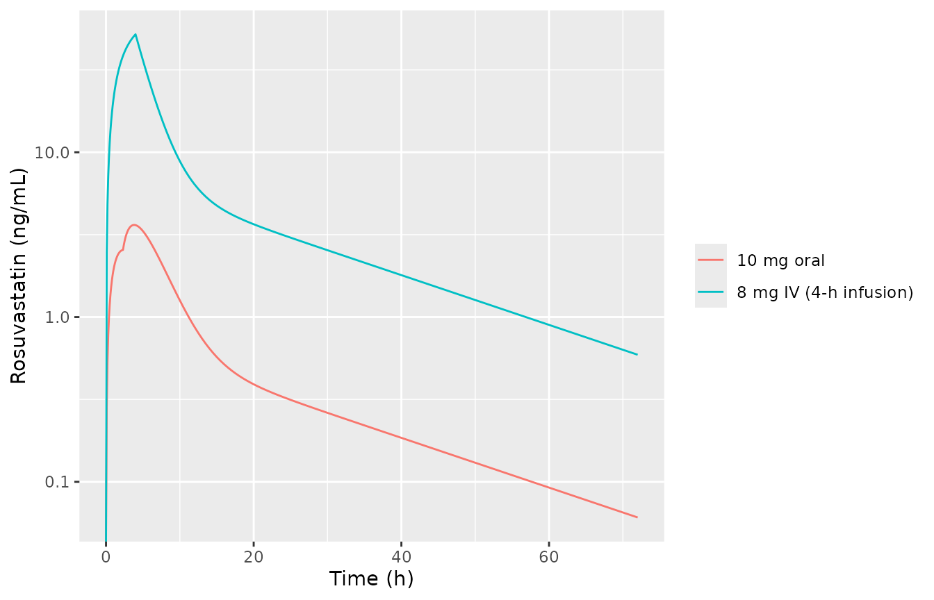
Typical-value rosuvastatin profiles. The shoulder in the oral profile at 2.3 h is the delayed second dose portion (compare Figure 1 of Hanke 2021).
Stochastic simulation
A cohort of 200 virtual subjects receives a single 10 mg fasted oral dose, the design of both oral training studies.
n_sub <- 200
ev_vpc <- dplyr::bind_rows(lapply(seq_len(n_sub), function(i) {
  oral_events(i, 10, "10 mg oral")
}))
rxode2::rxSetSeed(20211018)
sim_vpc <- rxode2::rxSolve(mod, ev_vpc, keep = "treatment", returnType = "data.frame")
#> ℹ parameter labels from comments will be replaced by 'label()'

vpc_band <- sim_vpc |>
  dplyr::group_by(time) |>
  dplyr::summarise(
    q05 = quantile(Cc, 0.05),
    q50 = quantile(Cc, 0.50),
    q95 = quantile(Cc, 0.95),
    .groups = "drop"
  )
ggplot(vpc_band, aes(time)) +
  geom_ribbon(aes(ymin = q05, ymax = q95), fill = "steelblue", alpha = 0.3) +
  geom_line(aes(y = q50), colour = "steelblue") +
  geom_hline(yintercept = c(4.48, 4.11), linetype = "dashed", colour = "grey40") +
  coord_cartesian(xlim = c(0, 48)) +
  labs(x = "Time (h)", y = "Rosuvastatin (ng/mL)")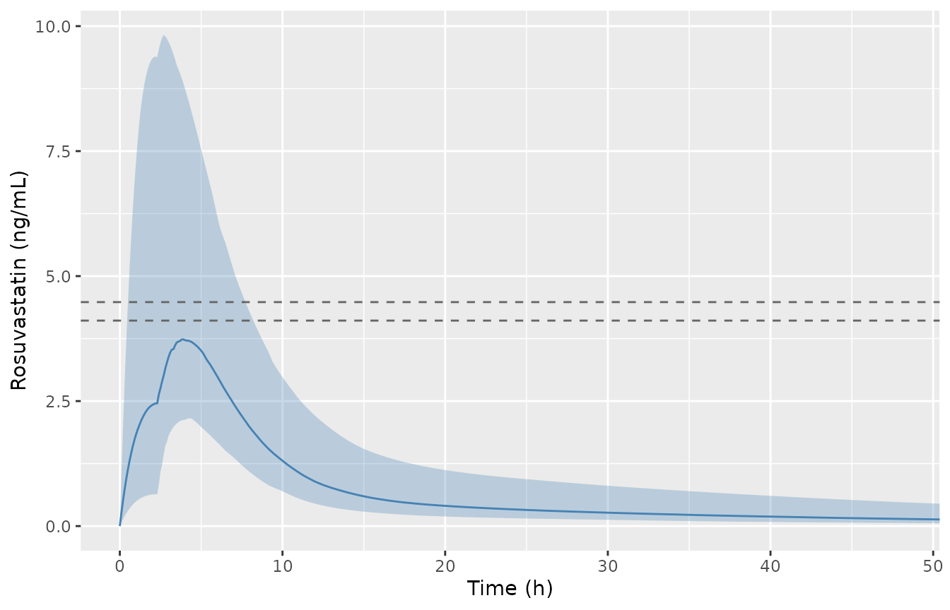
Median and 90% interval of 200 simulated subjects after 10 mg rosuvastatin orally (IPRED, without residual error). Dashed lines: observed Cmax of Stopfer et al. 2016 (4.48 ng/mL) and 2018b (4.11 ng/mL), ESM Table S3.5.2. Compare with the individual fits in ESM Figures S2.4.3-S2.4.6.
PKNCA validation
nca_for <- function(sim, events, conc_col) {
  conc <- sim |>
    dplyr::mutate(conc = .data[[conc_col]]) |>
    dplyr::filter(!is.na(conc)) |>
    dplyr::select(id, time, conc, treatment)
  # One dose row per id: for oral dosing the depot and depot2 records carry
  # the same full dose.
  dose <- events |>
    dplyr::filter(evid == 1) |>
    dplyr::distinct(id, time, amt, treatment)
  PKNCA::pk.nca(PKNCA::PKNCAdata(
    PKNCA::PKNCAconc(conc, conc ~ time | treatment + id),
    PKNCA::PKNCAdose(dose, amt ~ time | treatment + id),
    intervals = data.frame(
      start = 0, end = Inf,
      cmax = TRUE, tmax = TRUE, auclast = TRUE, aucinf.obs = TRUE, half.life = TRUE
    )
  ))
}

nca_typ <- as.data.frame(nca_for(sim_typ, ev_typ, "Cc")) |>
  dplyr::filter(PPTESTCD %in% c("cmax", "tmax", "auclast", "aucinf.obs", "half.life")) |>
  dplyr::select(treatment, PPTESTCD, PPORRES)

nca_vpc <- as.data.frame(nca_for(sim_vpc, ev_vpc, "Cc")) |>
  dplyr::filter(PPTESTCD %in% c("cmax", "tmax", "auclast")) |>
  dplyr::select(treatment, id, PPTESTCD, PPORRES)
Structural checks
The typical-value AUC0-inf has a closed form, Dose / CL
intravenously and FTOT * Dose / CL orally, whatever the
split fraction and lag. The terminal half-life is
ln 2 / beta, where beta is the smaller
eigenvalue of the two-compartment system. Both sides use the same
parameters, so the only difference is numerical error in the solve and
in the NCA extrapolation, and a tight bound is appropriate.
p <- list(cl = 19.1, vc = 79.4, q = 12.0, vp = 199, f = 0.0793)
k10 <- p$cl / p$vc
k12 <- p$q / p$vc
k21 <- p$q / p$vp
beta <- ((k10 + k12 + k21) - sqrt((k10 + k12 + k21)^2 - 4 * k10 * k21)) / 2

expected <- tibble::tibble(
  treatment = c("10 mg oral", "8 mg IV (4-h infusion)"),
  aucinf_expected = c(p$f * 10, 8) / p$cl * 1000,
  half_life_expected = log(2) / beta
)

check_typ <- nca_typ |>
  tidyr::pivot_wider(names_from = PPTESTCD, values_from = PPORRES) |>
  dplyr::left_join(expected, by = "treatment")

stopifnot(
  all(abs(check_typ$aucinf.obs / check_typ$aucinf_expected - 1) < 0.01),
  all(abs(check_typ$half.life / check_typ$half_life_expected - 1) < 0.02)
)

# The paper's split: 63.4% of the dose without lag, 36.6% after 2.3 h.
stopifnot(
  abs(plogis(log(0.366 / (1 - 0.366))) - 0.366) < 1e-12,
  abs(1 - 0.366 - 0.634) < 1e-12
)

knitr::kable(
  check_typ |>
    dplyr::select(treatment, cmax, tmax, aucinf.obs, aucinf_expected, half.life, half_life_expected) |>
    dplyr::rename(
      "Treatment" = treatment,
      "Cmax (ng/mL)" = cmax,
      "Tmax (h)" = tmax,
      "AUC0-inf (ng*h/mL)" = aucinf.obs,
      "Closed-form AUC0-inf" = aucinf_expected,
      "t1/2 (h)" = half.life,
      "Closed-form t1/2" = half_life_expected
    ),
  digits = 2,
  caption = "Typical-value NCA against the closed forms."
)| Treatment | Cmax (ng/mL) | Tmax (h) | AUC0-inf (ng*h/mL) | Closed-form AUC0-inf | t1/2 (h) | Closed-form t1/2 |
|---|---|---|---|---|---|---|
| 10 mg oral | 3.62 | 3.8 | 41.50 | 41.52 | 19.8 | 19.94 |
| 8 mg IV (4-h infusion) | 52.00 | 4.0 | 418.73 | 418.85 | 19.8 | 19.94 |
Comparison against published NCA
ESM Table S3.5.2 gives the observed AUClast and Cmax of every study in the paper; its “Pred” columns are PBPK predictions and are not used here. The two oral training studies of the population-PK model are compared with the median of the simulated 10 mg cohort. The simulated AUClast runs to 72 h. The ESM does not give the last sampling time, but the typical-value AUC grows by only about 2.5% between 72 and 96 h, so the choice hardly matters.
published <- tibble::tribble(
  ~study,                 ~cmax, ~auclast,
  "Stopfer et al. 2016",  4.48,  41.00,
  "Stopfer et al. 2018b", 4.11,  42.22
)

sim_nca <- nca_vpc |>
  dplyr::select(-id)

cmp <- dplyr::bind_rows(lapply(seq_len(nrow(published)), function(i) {
  nlmixr2lib::ncaComparisonTable(
    simulated = sim_nca |> dplyr::mutate(treatment = published$study[i]),
    reference = published[i, ] |> dplyr::rename(treatment = study),
    by = "treatment",
    units = c(cmax = "ng/mL", tmax = "h", auclast = "ng*h/mL"),
    tolerance_pct = 20
  )
}))

knitr::kable(
  cmp,
  caption = "Median of 200 simulated subjects (10 mg oral) vs. the observed values of the two oral training studies in Hanke 2021 ESM Table S3.5.2. * differs from the reference by more than 20%.",
  align = c("l", "l", "r", "r", "r")
)| NCA parameter | treatment | Reference | Simulated | % diff |
|---|---|---|---|---|
| Cmax (ng/mL) | Stopfer et al. 2016 | 4.48 | 3.79 | -15.3% |
| AUClast (ng*h/mL) | Stopfer et al. 2016 | 41 | 41.8 | +2.0% |
| Cmax (ng/mL) | Stopfer et al. 2018b | 4.11 | 3.79 | -7.7% |
| AUClast (ng*h/mL) | Stopfer et al. 2018b | 42.2 | 41.8 | -0.9% |
vpc_wide <- nca_vpc |>
  tidyr::pivot_wider(names_from = PPTESTCD, values_from = PPORRES)

r_auc <- median(vpc_wide$auclast) / published$auclast
r_cmax <- median(vpc_wide$cmax) / published$cmax

stopifnot(
  # AUC depends only on FTOT / CL for the oral route: a mis-transcribed
  # clearance, bioavailability or unit moves it by tens of percent.
  all(abs(r_auc - 1) < 0.2),
  # Cmax depends on ka, the split, the lag and the volumes; the observed
  # study summaries are not stated to be medians, so the tolerance is wider.
  all(abs(r_cmax - 1) < 0.3),
  # The median tmax reproduces the late peak described in the paper
  # (tmax = 5.0 h in the Results; typical-value 3.8 h here).
  median(vpc_wide$tmax) > 2.5,
  median(vpc_wide$tmax) < 6
)
The simulated median AUClast is within a few percent of both observed values. The simulated median Cmax runs below the observed values by about 8-15%. The observed values in Table S3.5.2 are study summaries (their statistic is not stated), and the 80% CV on the first-portion bioavailability makes a mean Cmax sit above the median.
Intravenous arm: a documented discrepancy
The same table gives the observed AUClast of the intravenous training
study, Martin et al. 2003c (8 mg over 4 h): 163.14 ngh/mL. The
model’s typical-value AUC0-inf for that dose is
8 / 19.1 * 1000 = 419 ngh/mL, about 2.5 times higher.
The observed data alone imply a bioavailability of about 0.20
(dose-normalised oral over intravenous AUClast), against the fitted FTOT
of 0.0793. The oral data pin only FTOT / CL. The printed CL
and FTOT are both about 2.5-fold lower than the data-only values, and
their ratio still matches, which is why the oral comparisons above agree
while the intravenous one does not. The ESM does not show the
population-PK fit to the intravenous profile (Figures S2.4.3-S2.4.8 show
only the oral and DDI subjects), so the cause cannot be identified from
the paper. The model is provided as published.
iv_auc_obs <- 163.14
oral_auc_obs <- mean(published$auclast)
iv_sim <- check_typ$aucinf.obs[check_typ$treatment == "8 mg IV (4-h infusion)"]
f_data <- (oral_auc_obs / 10) / (iv_auc_obs / 8)

knitr::kable(
  tibble::tibble(
    Quantity = c(
      "Typical IV AUC0-inf, model (ng*h/mL)",
      "Observed IV AUClast, Martin et al. 2003c (ng*h/mL)",
      "Ratio model / observed",
      "Data-only bioavailability (oral / IV, dose-normalised)",
      "Fitted FTOT"
    ),
    Value = c(iv_sim, iv_auc_obs, iv_sim / iv_auc_obs, f_data, 0.0793)
  ),
  digits = 3,
  caption = "The intravenous arm is not reproduced by the published CL and FTOT."
)| Quantity | Value |
|---|---|
| Typical IV AUC0-inf, model (ng*h/mL) | 418.725 |
| Observed IV AUClast, Martin et al. 2003c (ng*h/mL) | 163.140 |
| Ratio model / observed | 2.567 |
| Data-only bioavailability (oral / IV, dose-normalised) | 0.204 |
| Fitted FTOT | 0.079 |
# This locks in the documented discrepancy (deterministic typical-value
# solve). If the parameter values change, update this section.
stopifnot(iv_sim / iv_auc_obs > 2, iv_sim / iv_auc_obs < 3)
The DDI extension of the population-PK model
ESM section 2.4.1 also refits the model with the rifampicin, probenecid and gemfibrozil DDI study arms added. Covariate factors on bioavailability and clearance describe each interaction. During rifampicin and probenecid co-administration the dose is not split and has no lag time. The re-estimated typical values (“with DDI” column of Table S2.4.1) are shown below for reference. The DDI covariate factors themselves are not reported anywhere in the paper or ESM, and the control stream in section 2.4.2 is the model without DDI, so the DDI model is not provided.
| Parameter | Without DDI (this model) | With DDI |
|---|---|---|
| Ka (1/h) | 0.464 | 0.397 |
| Ftot (%) | 7.93 | 8.40 |
| VF2 | 0.366 | 0.338 |
| ALAG2 (h) | 2.30 | 2.26 |
| CL (L/h) | 19.1 | 18.9 |
| V3 (L) | 79.4 | 83.2 |
| Q (L/h) | 12.0 | 12.5 |
| V4 (L) | 199 | 211 |
| IIV Ftot (%CV) | 80.1 | 69.8 |
| IIV VF2 (%CV) | 77.8 | 64.8 |
| IIV CL (%CV) | 26.1 | 27.1 |
| Prop RE (%) | 22.2 | 26.9 |
| Add RE (ng/mL) | 0.00775 (fixed) | n.a. |
Assumptions and deviations
- Only the monotherapy population-PK model is provided. The PK-Sim whole-body PBPK model (including all DDI predictions) is not reproduced. Its partition coefficients, organ physiology and transporter expression are platform database outputs that the paper does not tabulate. The DDI extension of the population-PK model is not provided because its covariate factors are not reported (see above).
-
IIV “Ftot” acts on the first dose portion only.
Table S2.4.1 and the text describe IIV on the total bioavailability. The
control stream applies
EXP(ETA(3))toF1only (F2 = VF2_2 * FTOThas noETA(3)). The model follows the control stream. -
%CV to variance. Table S2.4.1 reports each IIV as a
%CV. The variances here use
omega^2 = log(1 + CV^2), the log-normal relation the ESM itself uses elsewhere (Table S7.0.1 footnote: “35 % CV was assumed (= 1.40 GeoSD)”). The same conversion is applied to the logit-scale VF2 eta. If the authors instead reported100 * sqrt(omega^2)for that row, the variance would be 0.605 rather than 0.473. The$OMEGAvalues printed in the control stream are initial estimates and were not used. -
Additive residual error. The control stream fixes
the additive
$SIGMAat 0.00006, i.e. an SD of 0.0077 ng/mL, matching Table S2.4.1. -
Concentration unit. The control stream scales the
central amount by
S3 = V3/1000with volumes in litres. With doses in mg this gives ng/mL, the unit of the additive error and of the observed values in Table S3.5.2. -
Intravenous arm. The published CL and FTOT do not
reproduce the observed intravenous AUClast (see above). Oral
predictions, which depend on
FTOT / CL, agree with the observed data. No parameter was adjusted. -
Dose records. An oral dose must be given as two
records of the full dose, to
depotanddepot2. A single record todepotalone would deliver only(1 - VF2) * FTOTof the dose.