Ceftiofur PK/PD against Pasteurella multocida in swine (Mi 2022)
Source:vignettes/articles/Mi_2022_ceftiofur.Rmd
Mi_2022_ceftiofur.RmdModel and source
Mi 2022 sets a dose of ceftiofur, a third-generation cephalosporin licensed only for veterinary use, against Pasteurella multocida in pigs. Ceftiofur is rapidly converted to desfuroylceftiofur (DFC), and every concentration in the paper is DFC. The paper has three quantitative components, and each is packaged as its own model file:
| Model file | What it is | Source |
|---|---|---|
Mi_2022_ceftiofur_pkpd_plasma |
Ex vivo inhibitory sigmoid Imax model, E vs AUC24h/MIC, plasma | Section 4.6, Table 3 |
Mi_2022_ceftiofur_pkpd_balf |
Same model fitted in bronchoalveolar lavage fluid (BALF) | Section 4.6, Table 3 |
Mi_2022_ceftiofur_semimech |
Semi-mechanistic growing/resting time-kill PD (fitted in vitro) driven by a one-compartment surrogate of the swine PBPK model | Section 4.8.2, Table 5, supplement Table S2 |
The plasma and BALF fits come from the same experiment but were fitted separately, so they ship as separate files. The semi-mechanistic model is the paper’s “PBPK/PD” model as it was simulated in Mlxplore: the PBPK model of Lin 2016 was first run at each dose, a one-compartment model was fitted to its unbound plasma output (supplement Table S2), and that compartmental PK drove the in vitro PD.
- Article: https://doi.org/10.3390/ijms23073722
- Supplement: https://www.mdpi.com/article/10.3390/ijms23073722/s1
m_plasma <- rxode2::rxode2(readModelDb("Mi_2022_ceftiofur_pkpd_plasma"))
m_balf <- rxode2::rxode2(readModelDb("Mi_2022_ceftiofur_pkpd_balf"))
m_semi <- rxode2::rxode2(readModelDb("Mi_2022_ceftiofur_semimech"))
Population
Six crossbred pigs (20 +/- 2 kg) were infected intranasally with P. multocida strain HB13 (Section 4.4) and then given a single intramuscular dose of ceftiofur hydrochloride, 5 mg/kg. Plasma was sampled from all six pigs from 0.33 to 96 h, and BALF from four of them from 0.33 to 48 h (Table 2). BALF concentrations were corrected for lavage dilution with the plasma:BALF urea ratio (supplement Table S1). HB13 has an MIC of 0.06 ug/mL and an MBC of 0.125 ug/mL, both in vitro and ex vivo (Section 2.1). The ex vivo time-kill curves (Figure 2) incubated about 5 x 10^6 CFU/mL of HB13 in each plasma or BALF sample for 24 h.
The semi-mechanistic PD was fitted to in vitro static time-kill curves in Mueller-Hinton broth: 10^6 CFU/mL of HB13 exposed to 1/4 to 8 x MIC, counted at 0, 3, 6, 9, 12 and 24 h in triplicate (Section 4.8.2, Figures 1 and 5). No animal covariates enter any of the three models, so no virtual cohort is needed. Every simulation below is a deterministic typical-value solve.
Source trace
| Quantity | Value | Source |
|---|---|---|
| Sigmoid Imax equation | E = E0 - Imax*INDEX^N/(INDEX^N + INDEX50^N) |
Section 4.6 |
| Imax, plasma / BALF | 9.78 / 7.41 log10 CFU/mL | Table 3 |
| E0, plasma / BALF | 3.57 / 3.59 log10 CFU/mL | Table 3 |
| IC50 (INDEX50), plasma / BALF | 60.14 / 59.84 h | Table 3 |
| N, plasma / BALF | 1.94 / 4.10 | Table 3 |
| MIC of HB13 | 0.06 ug/mL | Section 2.1 |
| Ex vivo inoculum | about 5 x 10^6 CFU/mL | Section 4.3.2 |
| PK: ka | 0.3381 1/h | Supplement Table S2 |
| PK: V/F | 1114.21 mL/kg (1114.11-1114.27 across doses) | Supplement Table S2 |
| PK: k | 0.0393 1/h | Supplement Table S2 |
| dG/dt, dR/dt | growing/resting ODEs | Section 4.8.2; supplement Equations 2-3 |
| kGR | (kgrowth - kdeath)*(G + R)/Bmax |
Section 4.8.2 (the supplement differs; see deviations) |
| EFFECT | Emax*C^gamma/(EC50^gamma + C^gamma) |
Section 4.8.2; supplement Equation 1 |
| kgrowth | 0.2 1/h | Table 5 |
| kdeath | 0.179 1/h (fixed) | Table 5 |
| Bmax | 8.48 log10 CFU/mL | Table 5 |
| Emax | 0.11 1/h | Table 5 |
| EC50 | 0.14 mg/L | Table 5 |
| gamma | 8.54 | Table 5 |
| In vitro inoculum | 10^6 CFU/mL | Section 4.8.2 |
Ex vivo sigmoid Imax models
The two ex vivo models take the 24 h AUC as the covariate
AUC_CEFTIOFUR. In the ex vivo design each sample holds one
fixed concentration for the 24 h incubation, so the AUC is simply 24 h
times that concentration. The index is
AUC_CEFTIOFUR / mic.
Table 3 target indices
Table 3 prints the AUC24h/MIC that gives no net change (E = 0), a 3-log10 kill (E = -3) and a 4-log10 kill (E = -4). Solving the model for those targets checks the transcription. The solve below runs the packaged models over a fine grid of exposures and interpolates the 24 h change.
grid_aucmic <- exp(seq(log(1), log(1000), length.out = 600))
ex_events <- function(aucmic) {
  data.frame(
    id = seq_along(aucmic), time = 24, evid = 0, amt = 0, cmt = "bact",
    AUC_CEFTIOFUR = aucmic * 0.06
  )
}
change_24h <- function(mod) {
  sim <- rxode2::rxSolve(mod, ex_events(grid_aucmic), returnType = "data.frame")
  sim$log_cfu - log10(5e6 + 1)
}
dE_plasma <- change_24h(m_plasma)
#> Warning: multi-subject simulation without without 'omega'
dE_balf <- change_24h(m_balf)
#> Warning: multi-subject simulation without without 'omega'

solve_target <- function(dE, target) {
  if (min(dE) > target) {
    return(NA_real_)
  }
  approx(dE, grid_aucmic, xout = target)$y
}
targets <- tibble::tribble(
  ~matrix, ~E, ~published,
  "Plasma", 0, 44.02,
  "Plasma", -3, 89.40,
  "Plasma", -4, 119.90,
  "BALF", 0, 58.99,
  "BALF", -3, 99.69,
  "BALF", -4, NA
) |>
  dplyr::rowwise() |>
  dplyr::mutate(
    model = solve_target(if (matrix == "Plasma") dE_plasma else dE_balf, E),
    pct_diff = 100 * (model - published) / published
  ) |>
  dplyr::ungroup()

targets |>
  dplyr::mutate(model = round(model, 2), pct_diff = round(pct_diff, 1)) |>
  dplyr::rename(
    "Matrix" = matrix, "Target E (log10 CFU/mL)" = E,
    "Published AUC24h/MIC (h)" = published, "Model AUC24h/MIC (h)" = model,
    "Difference (%)" = pct_diff
  ) |>
knitr::kable(caption = "Table 3 target indices, published versus solved from the packaged models.")| Matrix | Target E (log10 CFU/mL) | Published AUC24h/MIC (h) | Model AUC24h/MIC (h) | Difference (%) |
|---|---|---|---|---|
| Plasma | 0 | 44.02 | 45.21 | 2.7 |
| Plasma | -3 | 89.40 | 87.00 | -2.7 |
| Plasma | -4 | 119.90 | 113.48 | -5.4 |
| BALF | 0 | 58.99 | 58.94 | -0.1 |
| BALF | -3 | 99.69 | 99.49 | -0.2 |
| BALF | -4 | NA | NA | NA |
balf <- targets |> dplyr::filter(matrix == "BALF")
plasma <- targets |> dplyr::filter(matrix == "Plasma")
stopifnot(
  # BALF: both printed targets reproduce to better than 1%.
  all(abs(balf$pct_diff[!is.na(balf$published)]) < 1),
  # BALF: E0 - Imax = -3.82, so a 4-log10 kill is unreachable, which is why
  # Table 3 leaves that cell blank.
  is.na(balf$model[balf$E == -4]),
  # Plasma: within 6% (see the deviations section for why not closer).
  all(abs(plasma$pct_diff) < 6)
)
The BALF targets reproduce to within 0.2%. The plasma targets are within 3% for E = 0 and E = -3 and about 5% for E = -4. The printed plasma N of 1.94 is the cause: with E0 and Imax as printed, the three plasma targets are reproduced to better than 1% by N = 1.79 and IC50 = 60.0. Table 3 reports mean +/- SD, so the targets were probably averaged across animals separately from the curve parameters. The published values are kept.
Ex vivo kill at the plasma sample concentrations
Figure 2A lists the DFC concentration of each plasma sample. Two late samples straddle the effect range: 0.19 mg/L at 72 h and 0.05 mg/L at 96 h. Read from the figure, the 72 h sample fell from about 6.2 to about 3.5 log10 CFU/mL over 24 h (a change of about -2.7), and the 96 h sample grew to about 8.0 (about +1.8). These readings are approximate, taken by eye from the figure.
fig2a <- data.frame(sample = c("72 h (0.19 mg/L)", "96 h (0.05 mg/L)"), conc = c(0.19, 0.05), observed = c(-2.7, 1.8))
sim2a <- rxode2::rxSolve(
  m_plasma,
  data.frame(id = 1:2, time = 24, evid = 0, amt = 0, cmt = "bact", AUC_CEFTIOFUR = 24 * fig2a$conc),
  returnType = "data.frame"
)
#> Warning: multi-subject simulation without without 'omega'
fig2a$model <- round(sim2a$log_cfu - log10(5e6 + 1), 2)
fig2a |>
  dplyr::rename(
    "Plasma sample" = sample, "DFC (mg/L)" = conc,
    "Figure 2A change (log10 CFU/mL, read by eye)" = observed,
    "Model change (log10 CFU/mL)" = model
  ) |>
knitr::kable()| Plasma sample | DFC (mg/L) | Figure 2A change (log10 CFU/mL, read by eye) | Model change (log10 CFU/mL) |
|---|---|---|---|
| 72 h (0.19 mg/L) | 0.19 | -2.7 | -2.41 |
| 96 h (0.05 mg/L) | 0.05 | 1.8 | 2.54 |
Effect curves
data.frame(
  aucmic = rep(grid_aucmic, 2),
  change = c(dE_plasma, dE_balf),
  matrix = rep(c("Plasma", "BALF"), each = length(grid_aucmic))
) |>
  ggplot(aes(aucmic, change, colour = matrix)) +
  geom_line(linewidth = 1) +
  geom_hline(yintercept = c(0, -3, -4), linetype = "dashed", colour = "grey50") +
  scale_x_log10() +
  labs(x = "AUC24h/MIC (h)", y = "Change in log10 CFU/mL over 24 h", colour = NULL) +
  theme_bw()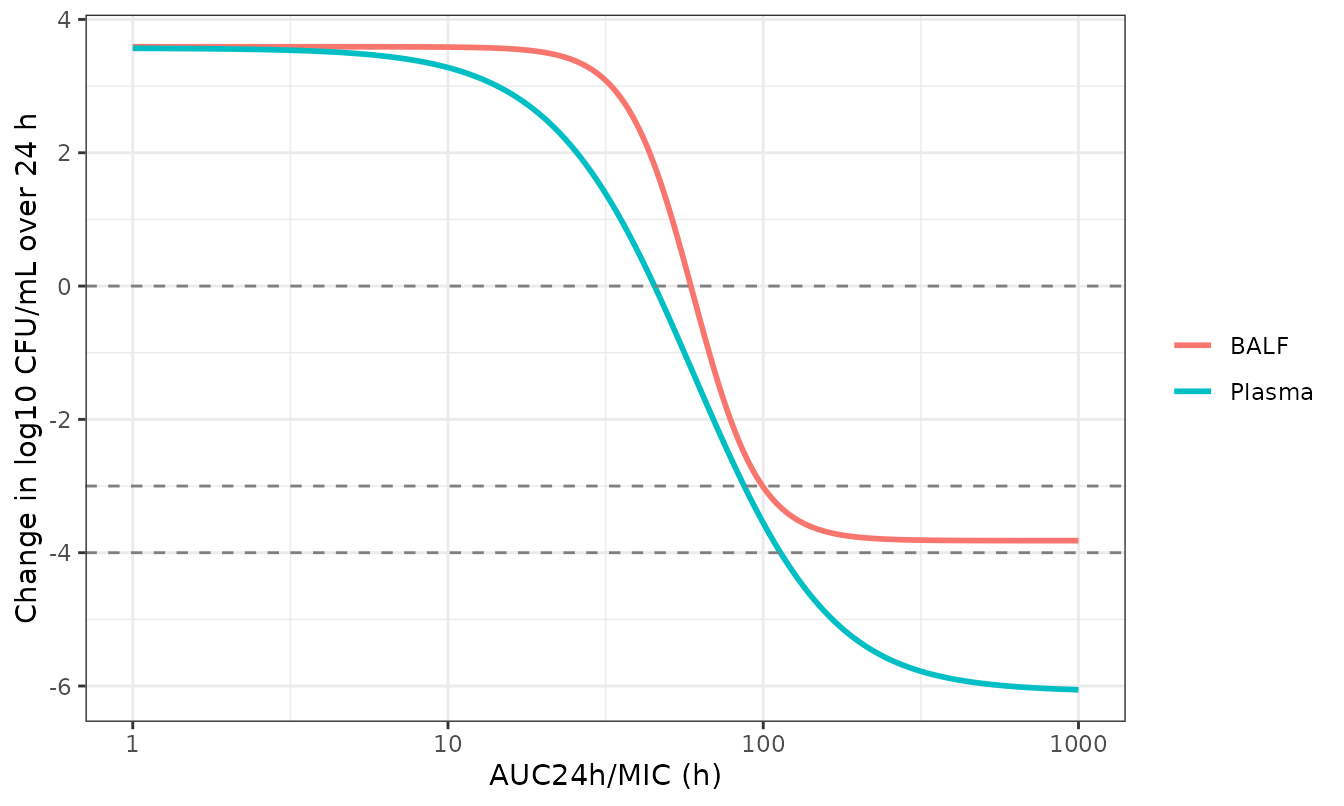
24 h change in bacterial count versus AUC24h/MIC for the plasma and BALF fits (Mi 2022 Table 3). Dashed lines mark the bacteriostatic, bactericidal and eradication levels.
Semi-mechanistic PK/PD model
PK layer (replicates Figure 6A and supplement Figure S1)
The three regimens are the doses the paper derived for bacteriostasis (0.22 mg/kg), bactericidal activity (0.46 mg/kg) and eradication (0.64 mg/kg).
doses <- c(0.22, 0.46, 0.64)
obs_times <- sort(unique(c(seq(0, 12, by = 0.25), seq(12, 72, by = 1))))
semi_events <- dplyr::bind_rows(lapply(seq_along(doses), function(i) {
  dplyr::bind_rows(
    data.frame(id = i, time = 0, evid = 1, amt = doses[i], cmt = "depot"),
    data.frame(id = i, time = obs_times, evid = 0, amt = 0, cmt = "central")
  )
}))
semi_sim <- rxode2::rxSolve(m_semi, semi_events, returnType = "data.frame") |>
  dplyr::mutate(regimen = paste(doses[id], "mg/kg"))
#> Warning: multi-subject simulation without without 'omega'
ggplot(semi_sim, aes(time, Cc, colour = regimen)) +
  geom_line(linewidth = 1) +
  labs(x = "Time (h)", y = "Unbound DFC (mg/L)", colour = NULL) +
  theme_bw()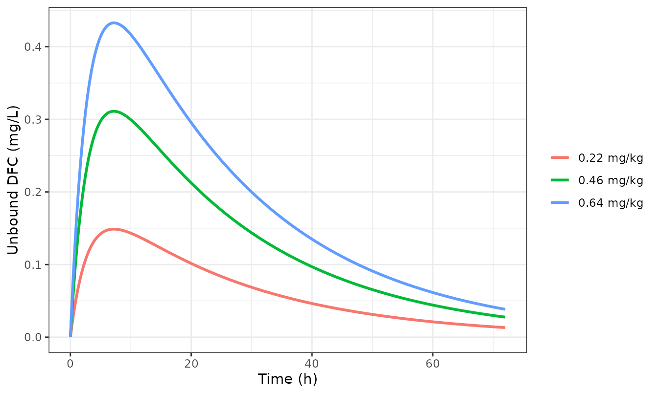
Replicates Figure 6A (and supplement Figure S1) of Mi 2022: unbound DFC plasma concentration after single intramuscular doses.
PKNCA validation of the PK layer
nca_in <- semi_sim |>
  dplyr::filter(!is.na(Cc)) |>
  dplyr::select(id, time, Cc, regimen)
stopifnot(all(nca_in$Cc[nca_in$time == 0] == 0))

conc_obj <- PKNCA::PKNCAconc(nca_in, Cc ~ time | regimen + id)
dose_obj <- PKNCA::PKNCAdose(
  semi_events |>
    dplyr::filter(evid == 1) |>
    dplyr::mutate(regimen = paste(amt, "mg/kg")) |>
    dplyr::select(id, time, amt, regimen),
  amt ~ time | regimen + id
)
intervals <- data.frame(start = 0, end = Inf, cmax = TRUE, tmax = TRUE, aucinf.obs = TRUE, half.life = TRUE)
nca_res <- PKNCA::pk.nca(PKNCA::PKNCAdata(conc_obj, dose_obj, intervals = intervals))

# Peaks read from supplement Figure S1 / Figure 6A.
published <- tibble::tribble(
  ~regimen, ~cmax, ~tmax,
  "0.22 mg/kg", 0.15, 7,
  "0.46 mg/kg", 0.31, 7,
  "0.64 mg/kg", 0.43, 7
)
cmp <- nlmixr2lib::ncaComparisonTable(
  simulated = nca_res,
  reference = published,
  by = "regimen",
  units = c(cmax = "mg/L", tmax = "h", aucinf.obs = "h*mg/L", half.life = "h"),
  tolerance_pct = 20
)
knitr::kable(cmp, caption = "Simulated PK versus the peaks read from Mi 2022 supplement Figure S1. * differs by >20%.")| NCA parameter | regimen | Reference | Simulated | % diff |
|---|---|---|---|---|
| Cmax (mg/L) | 0.22 mg/kg | 0.15 | 0.149 | -0.8% |
| Cmax (mg/L) | 0.46 mg/kg | 0.31 | 0.311 | +0.3% |
| Cmax (mg/L) | 0.64 mg/kg | 0.43 | 0.433 | +0.6% |
| Tmax (h) | 0.22 mg/kg | 7 | 7.25 | +3.6% |
| Tmax (h) | 0.46 mg/kg | 7 | 7.25 | +3.6% |
| Tmax (h) | 0.64 mg/kg | 7 | 7.25 | +3.6% |
nca_tab <- as.data.frame(nca_res)
vc <- 1.11421
kel <- 0.0393
auc_nca <- nca_tab |>
  dplyr::filter(PPTESTCD == "aucinf.obs") |>
  dplyr::arrange(id)
cmax_nca <- nca_tab |>
  dplyr::filter(PPTESTCD == "cmax") |>
  dplyr::arrange(id)
stopifnot(
  # One-compartment closed form: AUCinf = Dose / (V/F * k).
  all(abs(auc_nca$PPORRES / (doses / (vc * kel)) - 1) < 0.01),
  # Peaks read from Figure S1 (0.15, 0.31, 0.43 mg/L) to within 5%.
  all(abs(cmax_nca$PPORRES / c(0.15, 0.31, 0.43) - 1) < 0.05)
)
The PK surrogate reproduces the PBPK-predicted peaks of supplement
Figure S1. Its half-life, log(2)/0.0393 = 17.6 h, is longer
than the 13.3 h measured in the infected pigs after 5 mg/kg (Table 2,
which is total DFC by NCA). The surrogate describes the paper’s PBPK
simulation of unbound drug, not the observed data.
PD layer in vitro (compare Figures 1 and 5)
The PD parameters were estimated from static in vitro exposures. The
same model file reproduces a static bath by giving a bolus into
central plus an infusion that exactly replaces first-order
elimination, so Cc stays at the target concentration. The
PK layer is not changed.
mic <- 0.06
mults <- c(0, 0.25, 0.5, 1, 2, 4, 8)
invitro_events <- dplyr::bind_rows(lapply(seq_along(mults), function(i) {
  conc <- mults[i] * mic
  obs <- data.frame(id = i, time = seq(0, 24, by = 0.5), evid = 0, amt = 0, rate = 0, cmt = "central")
  if (conc == 0) {
    return(obs)
  }
  dplyr::bind_rows(
    data.frame(id = i, time = 0, evid = 1, amt = conc * vc, rate = 0, cmt = "central"),
    data.frame(id = i, time = 0, evid = 1, amt = conc * vc * kel * 24, rate = conc * vc * kel, cmt = "central"),
    obs
  )
}))
invitro_sim <- rxode2::rxSolve(m_semi, invitro_events, returnType = "data.frame") |>
  dplyr::mutate(arm = factor(ifelse(mults[id] == 0, "Control", paste0(mults[id], " x MIC")),
    levels = c("Control", paste0(mults[-1], " x MIC"))
  ))
#> Warning: multi-subject simulation without without 'omega'
# The bath concentration is held constant.
stopifnot(all(abs(invitro_sim$Cc - mults[invitro_sim$id] * mic) < 1e-6))
ggplot(invitro_sim, aes(time, log_cfu, colour = arm)) +
  geom_line(linewidth = 1) +
  labs(x = "Time (h)", y = "log10 CFU/mL", colour = NULL) +
  theme_bw()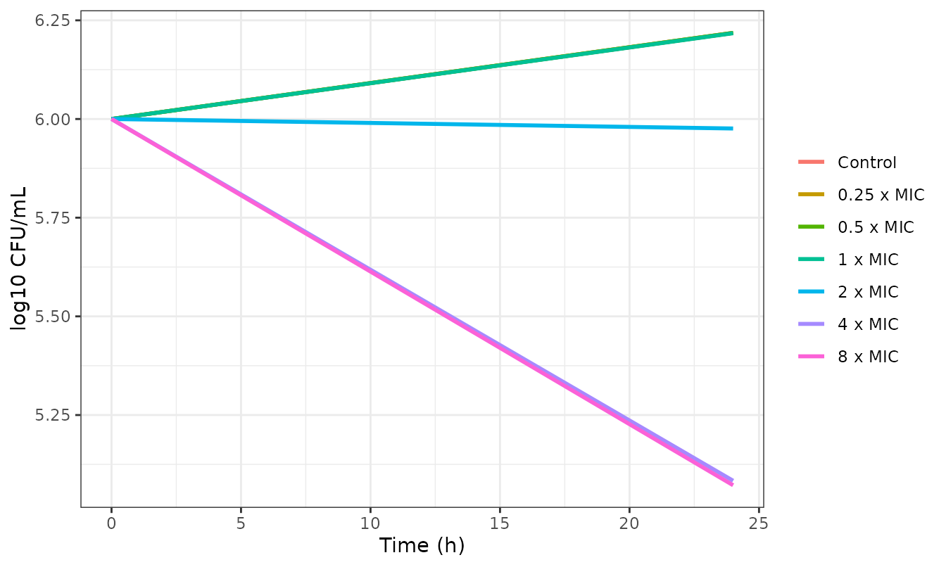
Typical-value in vitro time-kill predicted from Mi 2022 Table 5, for comparison with the observed means of Figure 1 and the individual fits of Figure 5.
fig1_24h <- c(9.1, 8.6, 7.9, 3.5, 2.0, 1.0, 1.0)
invitro_sim |>
  dplyr::filter(time == 24) |>
  dplyr::mutate(observed = fig1_24h[id], model = round(log_cfu, 2)) |>
  dplyr::select(arm, observed, model) |>
  dplyr::rename(
    "Exposure" = arm, "Observed at 24 h (read by eye, Figures 1 and 5)" = observed,
    "Model at 24 h (log10 CFU/mL)" = model
  ) |>
knitr::kable()| Exposure | Observed at 24 h (read by eye, Figures 1 and 5) | Model at 24 h (log10 CFU/mL) |
|---|---|---|
| Control | 9.1 | 6.22 |
| 0.25 x MIC | 8.6 | 6.22 |
| 0.5 x MIC | 7.9 | 6.22 |
| 1 x MIC | 3.5 | 6.22 |
| 2 x MIC | 2.0 | 5.98 |
| 4 x MIC | 1.0 | 5.08 |
| 8 x MIC | 1.0 | 5.07 |
The typical values do not reproduce the time-kill data; see the
deviations section. Two structural properties do hold and are checked
here. Over a long horizon the drug-free control plateaus at
Bmax = 10^8.48 CFU/mL, the fixed point of the main-text
kGR form. The initial net rate of change of the growing
state is kgrowth - kdeath - EFFECT.
long_ctl <- rxode2::rxSolve(
  m_semi,
  data.frame(id = 1, time = c(0, 5000), evid = 0, amt = 0, cmt = "central"),
  returnType = "data.frame"
)
early <- invitro_sim |> dplyr::filter(time %in% c(0, 0.5))
early_rate <- early |>
  dplyr::group_by(id) |>
  dplyr::summarise(rate = diff(log_cfu) * log(10) / 0.5)
c_bath <- mults * mic
expected_rate <- 0.2 - 0.179 - 0.11 * c_bath^8.54 / (0.14^8.54 + c_bath^8.54)
stopifnot(
  abs(long_ctl$log_cfu[2] - 8.48) < 0.01,
  all(abs(early_rate$rate - expected_rate) < 0.005)
)
PD layer driven by the PK (replicates Figure 6B)
ggplot(semi_sim, aes(time, log_cfu, colour = regimen)) +
  geom_line(linewidth = 1) +
  labs(x = "Time (h)", y = "log10 CFU/mL", colour = NULL) +
  theme_bw()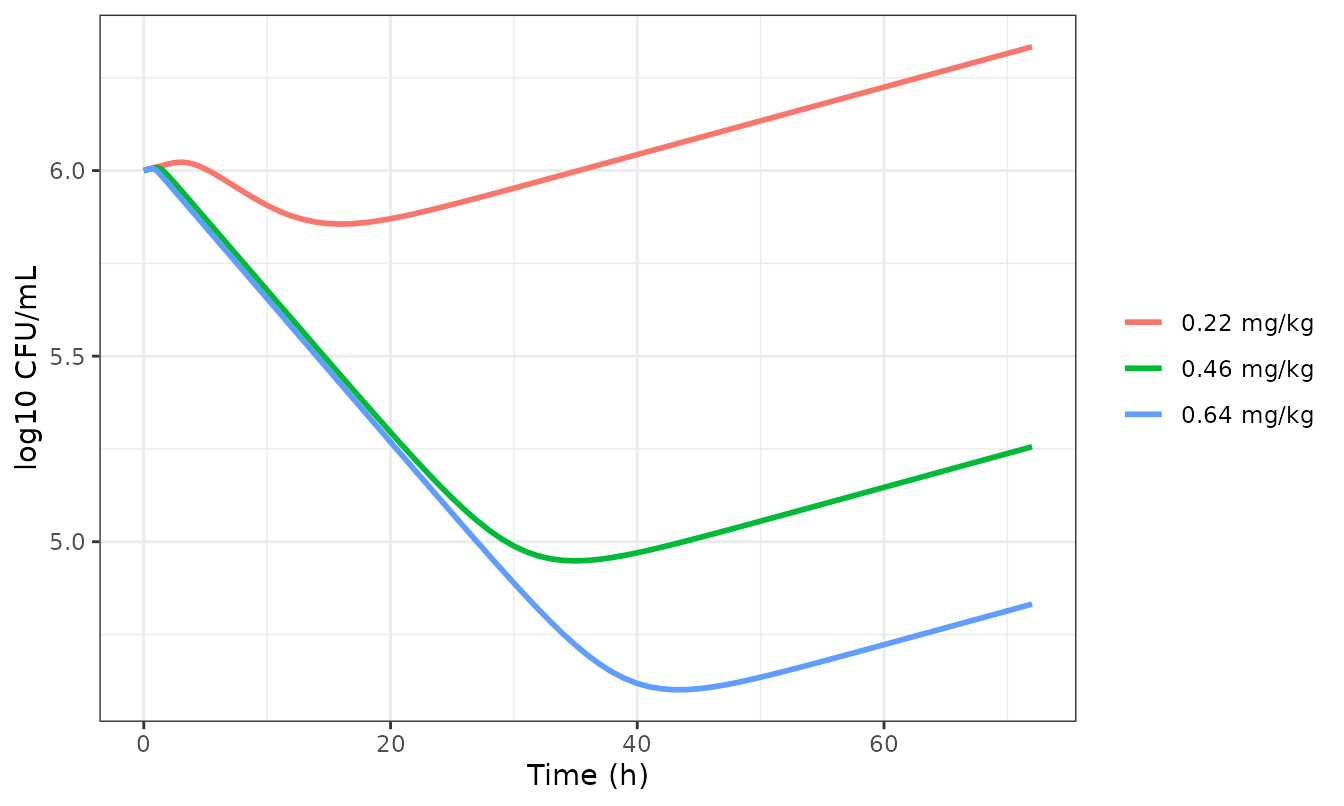
Replicates the layout of Mi 2022 Figure 6B: typical-value bacterial count under the three single intramuscular doses. The paper’s own curves fall much further (see the table below).
fig6b <- tibble::tribble(
  ~regimen, ~paper_min, ~paper_72,
  "0.22 mg/kg", 4.3, 5.8,
  "0.46 mg/kg", 0.4, 0.7,
  "0.64 mg/kg", 0.2, 0.2
)
semi_sim |>
  dplyr::group_by(regimen) |>
  dplyr::summarise(model_min = round(min(log_cfu), 2), model_72 = round(log_cfu[time == 72], 2)) |>
  dplyr::left_join(fig6b, by = "regimen") |>
  dplyr::select(regimen, paper_min, model_min, paper_72, model_72) |>
  dplyr::rename(
    "Dose" = regimen,
    "Figure 6B minimum (read by eye)" = paper_min, "Model minimum" = model_min,
    "Figure 6B at 72 h (read by eye)" = paper_72, "Model at 72 h" = model_72
  ) |>
knitr::kable(caption = "log10 CFU/mL: Mi 2022 Figure 6B versus the packaged Table 5 typical values.")| Dose | Figure 6B minimum (read by eye) | Model minimum | Figure 6B at 72 h (read by eye) | Model at 72 h |
|---|---|---|---|---|
| 0.22 mg/kg | 4.3 | 5.86 | 5.8 | 6.33 |
| 0.46 mg/kg | 0.4 | 4.95 | 0.7 | 5.26 |
| 0.64 mg/kg | 0.2 | 4.60 | 0.2 | 4.83 |
Assumptions and deviations
-
The Table 5 PD parameters do not reproduce the paper’s own
figures. With
kgrowth= 0.2 andkdeath= 0.179 1/h the drug-free net growth rate is only 0.021 1/h. The typical-value control therefore grows 0.2 log10 in 24 h, against about 3 log10 in Figure 1 and in the control panel of Figure 5. WithEmax= 0.11 1/h the fastest possible net kill is 0.089 1/h, about 0.9 log10 per 24 h. The observed 4 and 8 x MIC arms fall about 5 log10 in 24 h. In Figure 6B the 0.46 and 0.64 mg/kg doses reach 0.2-0.7 log10 CFU/mL by 72 h, but the typical values give about 5 log10 CFU/mL. The Table 5 values agree with the paper’s text:Emax/kdeath= 0.61 matches the “0.6-fold increase in death rate”, andEC50/MIC= 2.3 matches the “2.3-fold of MIC”. Supplement Figure S2 shows a poor population-prediction fit next to a good individual-prediction fit. That points to large between-experiment variability, whose magnitude is not reported. The standard error ofkgrowth(0.28) also exceeds the estimate. Figure 5 plots individual predictions, which would explain why those fits look good. It does not explain Figure 6B, a deterministic simulation. No reading of the published values reproduces it, and the values are shipped as published, without tuning. -
Bmaxunits. Table 5 prints the unit ofBmaxas 1/h, copied from the rows above it.Bmaxis the maximum bacterial concentration. The value 8.48 is read as log10 CFU/mL (3.0 x 10^8 CFU/mL), as in the original Nielsen 2007 model. Read literally as 8.48 CFU/mL, the resting-state transfer would drive every culture, including the controls, to extinction. -
kGRform. The main text (Section 4.8.2) printskGR = (kgrowth - kdeath) * (G + R) / Bmax, the Nielsen 2007 form. The supplement’s Equation section prints(kgrowth - kdeath) * (1 - (G + R) / Bmax), which has no carrying capacity: atG + R = Bmaxthe transfer stops and the growing state keeps growing, so the controls would never plateau as they do in Figure 1. The main-text form is used. -
gamma. Table 5 prints no standard error forgamma(8.54), but marks onlykdeathas “(fixed)”.gammais treated as estimated. This does not affect simulation. -
PK layer. The PK is the one-compartment surrogate
of supplement Table S2, not the Lin 2016 whole-body PBPK model itself.
The three per-dose fits share
kaandk, and their V/F values differ only in the fifth significant figure (1114.11, 1114.27, 1114.21 mL/kg). The 0.64 mg/kg value, the middle of the three, is used. The PK predicts the unbound DFC concentration (Section 4.8.1 and Figure 4), and that is the concentration the PD sees. The paper does not print the Lin 2016 PBPK equations, and its Monte Carlo analysis (Table 4, Figure 4) only varies that model’s inputs, so neither is reproduced here. -
No variability or residual error. None of the three
fits reports between-animal or between-experiment variances or a
residual error. The +/- values in Table 3 are SDs of the estimates. All
three models are typical-value only, with
addSdfixed at 0. - Plasma target indices. The Table 3 plasma targets reproduce to 3-5% rather than to the rounding error that the BALF targets achieve. The plasma targets and curve parameters appear to have been summarised separately (Table 3 is mean +/- SD). The printed parameters are kept.
- Initial inoculum. The ex vivo models start at 5 x 10^6 CFU/mL (Section 4.3.2) and the in vitro model at 10^6 CFU/mL (Section 4.8.2). The ex vivo models predict a change over 24 h, which does not depend on the starting count.
- Figure readings. Every “read by eye” value in this article was read from the published figures and is approximate. It is used for comparison only, never to set a parameter.