Leuprorelin, testosterone and PSA (Snelder 2019)
Source:vignettes/articles/Snelder_2019_leuprorelin.Rmd
Snelder_2019_leuprorelin.RmdModels and source
Snelder 2019 fits three separate leuprorelin PK models, one per depot formulation, and one testosterone (T) - prostate specific antigen (PSA) pharmacodynamic model. The T-PSA model was developed on study EC403 (the 6-month depot) and then applied unchanged, with its parameters fixed, to the other studies. The library therefore carries three model files:
| Model | Study / formulation | Contents |
|---|---|---|
Snelder_2019_leuprorelin |
EC403, 6-month depot 22.5 / 30 mg | joint PK + T + PSA |
Snelder_2019_leuprorelin_1m |
EC402, 1-month depot 3.75 mg | PK only |
Snelder_2019_leuprorelin_4m |
EC402, 4-month depot 15 mg | PK only |
- Citation: Snelder N, Drenth HJ, Riber Bergmann K, Wood ND, Hibberd M, Scott G. Population pharmacokinetic-pharmacodynamic modelling of the relationship between testosterone and prostate specific antigen in patients with prostate cancer during treatment with leuprorelin. Br J Clin Pharmacol. 2019;85(6):1247-1259. doi:10.1111/bcp.13891. Structural equations from Methods 2.5-2.6 (Equations 1, 4, 5, 7); parameter values from Tables 2-4; the NONMEM control stream in Supplement 4 resolves the terms the main text leaves implicit.
- Article: https://doi.org/10.1111/bcp.13891
- Supplements 1-5 (PK models for EC402 and EC404, individual fits, the NONMEM control stream, and the eta distributions) are attached to the article at the same DOI.
mod_6m <- readModelDb("Snelder_2019_leuprorelin")
mod_1m <- readModelDb("Snelder_2019_leuprorelin_1m")
mod_4m <- readModelDb("Snelder_2019_leuprorelin_4m")

ui_6m <- rxode2::rxode(mod_6m)
ui_1m <- rxode2::rxode(mod_1m)
ui_4m <- rxode2::rxode(mod_4m)

# Typical-value (zeroRe) counterparts used for every deterministic check.
tv_6m <- mod_6m |> rxode2::zeroRe()
tv_1m <- mod_1m |> rxode2::zeroRe()
tv_4m <- mod_4m |> rxode2::zeroRe()

# Typical values, pulled from the packaged model rather than retyped, so the
# closed-form checks below cannot drift away from the shipped ini().
theta <- function(ui, nm) {
  v <- ui$theta[[nm]]
  stopifnot(length(v) == 1L, !is.na(v))
  v
}
p6 <- vapply(
  c("lcl", "lvc", "lq", "lvp", "lka_fast", "lka_slow", "lka_slope",
    "logitfrel", "lfdepot", "agonist_kd_ratio", "ldr50", "lhill_dr", "lkd",
    "lkout_tt", "lrbase_tt", "lrbase_rt", "lcpa", "lrbase_psa", "lkout_psa",
    "lemax", "lec50", "lhill_psa", "boxcox_lrbase_psa"),
  function(nm) theta(ui_6m, nm), numeric(1)
)
Population
Study EC403 randomised 62 Caucasian men with prostate cancer (mean age 70.5 years) from 71 screened, 31 to each of a 22.5 mg and a 30 mg leuprorelin-SR 6-month depot; 59 completed. Eighty-four percent were newly diagnosed, the remainder enrolled after a PSA relapse following radical prostatectomy or radiotherapy. Ninety percent received cyproterone acetate (CPA) 7 to 3 days before the first leuprorelin dose as flare prophylaxis (Methods 2.1, Results 3.2, Table 1).
Study EC402 enrolled 26 patients on the 3.75 mg 1-month depot (mean age 71.1 years, range 53-85) and 106 on the 15 mg 4-month depot (mean age 72.0 years, range 53-85), all with biopsy-confirmed prostate cancer requiring chemical castration, PSA at least 1 ng/mL and serum testosterone at least 150 ng/dL.
EC403 had the densest sampling and was used for model development; EC402, EC404 Stratum 2 and the Bruchovsky cohort were used only for external evaluation (Methods 2.3).
pop <- rxode2::rxode(mod_6m)$population
tibble::tibble(
  Field = names(pop),
  Value = vapply(pop, function(x) paste(
    if (is.null(names(x))) x else paste0(names(x), " = ", x),
    collapse = "; "
  ), character(1))
) |>
knitr::kable(caption = "EC403 population metadata carried by the model file.")| Field | Value |
|---|---|
| species | human |
| n_subjects | 62 |
| n_studies | 1 |
| age_range | not reported; mean 70.5 years |
| age_median | mean 70.5 years |
| sex_female_pct | 0 |
| race_ethnicity | White = 100 |
| disease_state | Prostate cancer; 83.9% newly diagnosed, the remainder enrolled for PSA relapse after radical prostatectomy or radiotherapy |
| dose_range | Single 22.5 mg or 30 mg leuprorelin-SR 6-month depot (31 subjects each) |
| co_medication | Cyproterone acetate (injection or oral) 7 to 3 days before the first leuprorelin dose in at-risk subjects; 90% of subjects received it |
| regions | not reported |
| notes | Study EC403: randomised, open-label, multicentre, parallel-group PK/PD study of two leuprorelin-SR 6-month depot doses (Methods 2.1 and Table 1). 62 Caucasian men randomised from 71 screened; 59 completed (28 in the 30 mg and 31 in the 22.5 mg group). EC403 had the densest sampling scheme and was used for model development; studies EC402, EC404 Stratum 2 and the Bruchovsky cohort were used only for external evaluation. Assay LOQs: leuprorelin 16 pg/mL (10.7% BLQ, M4 method), testosterone 10 ng/dL (21.9% BLQ, M3 method), PSA 0.1 ng/mL (4.5% BLQ, M3 method). The EC402 1-month and 4-month depot PK models are packaged separately as Snelder_2019_leuprorelin_1m and Snelder_2019_leuprorelin_4m. |
Source trace
Every ini() entry in the three model files carries an
in-file comment naming its source location. The tables below collect
them.
Leuprorelin PK, study EC403 6-month depot
(Snelder_2019_leuprorelin)
| Equation / parameter | Value | Source location |
|---|---|---|
lcl |
17.4 L/h | Table 2, CL (RSE 4.33%) |
lvc |
137 L | Table 2, Vc (RSE 6.15%) |
lq |
3.81 L/h | Table 2, Q (RSE 6.67%) |
lvp |
28.1 L | Table 2, Vp (RSE 11.6%) |
lka_fast |
1.57 1/h | Table 2, Ka1 (RSE 9.81%) |
lka_slow |
0.000361 1/h | Table 2, Ka2 (RSE 9.72%) |
lka_slope |
0.331e-6 1/h^2 | Table 2, Ka3_SLP (x 10^-6) (RSE 11.5%) |
logitfrel |
-0.218 (logit) | Table 2, Fr (RSE 26.5%); footnote a gives the 0.55 slow fraction |
lfdepot |
1, fixed | Supplement 4 $PK, RBIO = IRBIO ; 1
|
| mixture proportion | 0.408 | Table 2, prop Pop1 (RSE 18.9%); recorded in
covariateData$MIX_RAMP_REL$notes
|
| IIV RBIO / CL / Fr / (Ka2 & Ka3_SLP) | 0.127 / 0.0304 / 0.116 / 0.232 | Table 2, random effects |
propSd |
sqrt(0.303) = 0.5505 | Table 2, sigma^2 prop |
| two parallel release depots, 2-cmt disposition | n/a | Figure 1; Results 3.1; Supplement 4 $MODEL /
$DES
|
Testosterone model (Snelder_2019_leuprorelin)
| Equation / parameter | Value | Source location |
|---|---|---|
agonist_kd_ratio |
1, fixed | Methods 2.5 (GnRH “arbitrarily fixed to 1”) |
ldr50 |
0.0486 | Table 3, DR50 (RSE 22.6%) |
lhill_dr |
2.05 | Table 3, nHT (RSE 9.90%) |
lkd |
4.36 pg/mL | Table 3, Kd (RSE 36.5%) |
lkout_tt |
0.0164 1/h | Table 3, KoutT (RSE 4.02%) |
lrbase_tt |
449 ng/dL | Table 3, BSLT (RSE 4.68%) |
lrbase_rt |
1, fixed | Methods 2.5 (baseline receptor concentration set to 1) |
lcpa |
4.13 | Table 3, CPA (RSE 17.1%) |
| 6x6 IIV block (DR50, Kd, KoutT, BSLT, CPA, nHT) | 6 variances, 15 covariances | Table 3, random effects |
propSd_TT |
sqrt(0.0761) = 0.2759 | Table 3, sigma^2 prop |
FRAC_0, FRAC, DRR,
dRT/dt, RAC, dT/dt
|
n/a | Equation 1 (Methods 2.5) |
KoutT = KoutR;
KinT = KoutT*BSLT*KoutR/(FRAC0*KinR); DR
guard |
n/a | Supplement 4 $PK and $DES
|
| CPA window (336 h opening 168 h pre-dose) | n/a | Methods 2.5 (“assumed to last for 2 weeks”); Supplement 4
$DES START / END |
PSA model (Snelder_2019_leuprorelin)
| Equation / parameter | Value | Source location |
|---|---|---|
lrbase_psa |
9.73 ng/mL | Table 4, BSLP (RSE 4.68%) |
lkout_psa |
0.00241 1/h | Table 4, KoutP (RSE 5.81%) |
lemax |
57.3 | Table 4, Emax (RSE 20.4%) |
lec50 |
596 ng/dL | Table 4, EC50 (RSE 13.9%) |
lhill_psa |
2.49 | Table 4, nHP (RSE 13.8%) |
boxcox_lrbase_psa |
0.642 | Table 4, Box-Cox shape (RSE 7.29%) |
| 3x3 IIV block (KoutP, Emax, EC50) + nHP fixed + BSLP | Table 4 | Table 4, random effects |
propSd_PSA |
sqrt(0.0658) = 0.2565 | Table 4, sigma^2 prop |
dPSA/dt = KinP*(1 + EFF) - KoutP*PSA |
n/a | Equation 4 (Model 2) |
EFF = Emax*T^nHP/(EC50^nHP + T^nHP) |
n/a | Equation 5 |
KinP from the pre-treatment steady state |
n/a | Equation 7 |
| Box-Cox eta form | n/a | Supplement 4 $PK,
BSLP = THETA(2)*EXP(((EXP(ETA(5)))**THETA(7)-1)/THETA(7))
|
EC402 PK models
| Equation / parameter | 1-month 3.75 mg | 4-month 15 mg | Source location |
|---|---|---|---|
lcl |
21.7 L/h | 20.5 L/h | Tables S1.1 / S1.2 |
lvc |
219 L | 215 L | Tables S1.1 / S1.2 |
lq |
4.71 L/h | 4.98 L/h | Tables S1.1 / S1.2 |
vp |
fixed to Vc | fixed to Vc | Tables S1.1 / S1.2 |
lka_fast |
0.690 1/h | 0.480 1/h | Tables S1.1 / S1.2, Ka1 |
lka_slow |
n/a | 0.00464 1/h | Table S1.2, Ka2 |
ltlag |
n/a | 160 h | Table S1.2, Lag time |
lka_slope |
9.83e-6 1/h^2 | 0.757e-6 1/h^2 | Tables S1.1 / S1.2, Ka3_SLP (x 10^-6) |
ld1 |
803 h | 2880 h, fixed | Tables S1.1 / S1.2, Dsa |
| release fractions |
lfrel = 0.441 (natural scale) |
logitfrel = -0.799, logitfrel2 =
-1.62 |
Table footnotes |
lfdepot |
1, fixed | 1, fixed | Tables S1.1 / S1.2, RBIO |
propSd |
sqrt(0.0787) = 0.2805 | sqrt(0.142) = 0.3768 | Tables S1.1 / S1.2 |
| depot topology | Figure S1.1A | Figure S1.1B | Supplement 1 |
Structural checks in closed form
The paper reports no NCA table for leuprorelin, so the sharpest available checks are the algebraic identities the model is built on together with the percentages the paper states in prose. Each of these is deterministic: it compares two expressions evaluated from the same shipped parameters, so a tight tolerance is appropriate and is what makes the check catch a transcription error.
agn    <- p6[["agonist_kd_ratio"]]
cpa    <- exp(p6[["lcpa"]])
bslt   <- exp(p6[["lrbase_tt"]])
bslp   <- exp(p6[["lrbase_psa"]])
emax   <- exp(p6[["lemax"]])
ec50   <- exp(p6[["lec50"]])
nhp    <- exp(p6[["lhill_psa"]])
frel   <- plogis(p6[["logitfrel"]])

# Baseline receptor activation, Equation 1: FRAC_0 = GnRH / (1 + GnRH).
frac0 <- agn / (1 + agn)

# Cyproterone acetate divides the endogenous agonist activity by (1 + CPA)
# (Supplement 4 $DES, AGNN = AGN / (1 + CPA)). Results 3.2 states the
# consequences: "The CPA effect resulted in an 80.5% reduction in endogenous
# GnRH levels and, consequently, in a 67.3% reduction in endogenous T
# concentrations."
agn_cpa   <- agn / (1 + cpa)
frac_cpa  <- agn_cpa / (1 + agn_cpa)
gnrh_drop <- 100 * (1 - agn_cpa / agn)
t_drop    <- 100 * (1 - frac_cpa / frac0)

# Testosterone-driven stimulation of PSA production, Equation 5.
eff <- function(tt) emax * tt^nhp / (ec50^nhp + tt^nhp)

# Minimal steady-state PSA (Equation 9 with Tss -> 0) equals KinP / KoutP,
# and Equation 7 gives KinP / KoutP = BSLP / (1 + EFF(BSLT)).
psa_min <- bslp / (1 + eff(bslt))

# Results 3.4 / Discussion: the T level below which PSA no longer falls is the
# T at which the minimum is at least 95% of the steady-state PSA, i.e.
# PSAss(T) = PSA_min / 0.95.  Median reported: 35 ng/dL (95% CI 18-55).
t_target <- stats::uniroot(
  function(tt) (1 + eff(tt)) - 1 / 0.95, c(1, 400)
)$root

# Table 2 footnote a: the SLOW release fraction is 1 - expit(Fr) = 0.55.
slow_fraction <- 1 - frel

tibble::tibble(
  Check = c(
    "Baseline GnRH-receptor activation FRAC_0",
    "Reduction in endogenous GnRH activity from CPA (%)",
    "Reduction in typical testosterone from CPA (%)",
    "Slow-release dose fraction",
    "Typical minimal steady-state PSA (ng/mL)",
    "T at which PSA is within 5% of its minimum (ng/dL)"
  ),
  Model = c(frac0, gnrh_drop, t_drop, slow_fraction, psa_min, t_target),
  Paper = c(0.5, 80.5, 67.3, 0.55, NA, 35),
  Source = c(
    "Methods 2.5 (GnRH fixed to 1 implies 50% activity)",
    "Results 3.2", "Results 3.2", "Table 2 footnote a",
    "no typical value published; simulated median 0.62 with IIV (Results 3.4)",
    "Results 3.4 / Abstract (median 35, 95% CI 18-55)"
  )
) |>
  dplyr::mutate(dplyr::across(c(Model, Paper), \(x) signif(x, 4))) |>
knitr::kable(caption = "Closed-form reproduction of the values Snelder 2019 states in prose.")| Check | Model | Paper | Source |
|---|---|---|---|
| Baseline GnRH-receptor activation FRAC_0 | 0.5000 | 0.50 | Methods 2.5 (GnRH fixed to 1 implies 50% activity) |
| Reduction in endogenous GnRH activity from CPA (%) | 80.5100 | 80.50 | Results 3.2 |
| Reduction in typical testosterone from CPA (%) | 67.3700 | 67.30 | Results 3.2 |
| Slow-release dose fraction | 0.5543 | 0.55 | Table 2 footnote a |
| Typical minimal steady-state PSA (ng/mL) | 0.4878 | NA | no typical value published; simulated median 0.62 with IIV (Results 3.4) |
| T at which PSA is within 5% of its minimum (ng/dL) | 35.9600 | 35.00 | Results 3.4 / Abstract (median 35, 95% CI 18-55) |
stopifnot(
  # Exact by construction with GnRH = 1.
  abs(frac0 - 0.5) < 1e-12,
  # Both percentages are printed to one decimal, so agreement to 0.1 is the
  # tightest bound the printed precision supports.
  abs(gnrh_drop - 80.5) < 0.1,
  abs(t_drop - 67.3) < 0.1,
  # Table 2 footnote a prints 0.55 to two decimals.
  abs(slow_fraction - 0.55) < 0.005,
  # The paper rounds its headline threshold to 35 ng/dL and gives a 95% CI of
  # 18-55 from parameter uncertainty; the typical-value root must land inside
  # that CI and close to the headline.
  t_target > 18, t_target < 55, abs(t_target - 35) < 2
)
The typical-value minimal PSA of 0.488 ng/mL sits below the 0.62 ng/mL median the paper simulates (Results 3.4), which is expected: the baseline-PSA random effect is Box-Cox transformed with a positive shape parameter and the reported median is taken over that distribution, not at the typical value. The corresponding cohort median is checked below.
The three phases of the testosterone response
Figure 3 of the paper marks three phases in the EC403 testosterone
data: a CPA-driven decrease before leuprorelin (green), the agonist
flare (blue), and the receptor-downregulation-driven suppression
(orange). The event tables put time = 0 at the start of the
assumed CPA window, so the leuprorelin dose falls at 168 h and the CPA
effect is in force over [0, 336) h - the window Supplement
4’s $DES block encodes.
ec403_outputs <- c("Cc", "TT", "PSA")
T_DOSE   <- 168    # h; leuprorelin dose, 7 days after the CPA window opens
CPA_DUR  <- 336    # h; assumed duration of the CPA effect (Methods 2.5)

# Build an EC403 event table. `subj` carries one row per subject with columns
# id, dose_mg, cpa_flag (0/1) and MIX_RAMP_REL (0/1).
make_ec403_events <- function(subj, obs_times) {
  dose <- tidyr::crossing(subj, cmt = c("depot", "depot2")) |>
    dplyr::mutate(time = T_DOSE, evid = 1L, amt = dose_mg, rate = NA_real_)
  obs <- tidyr::crossing(subj, time = obs_times, cmt = ec403_outputs) |>
    dplyr::mutate(evid = 0L, amt = 0, rate = NA_real_)
  dplyr::bind_rows(dose, obs) |>
    dplyr::mutate(
      CONMED_CYPROTERONE = cpa_flag * as.numeric(time < CPA_DUR)
    ) |>
    dplyr::arrange(id, time, evid) |>
    as.data.frame()
}

# One observation row per (id, time) after the solve: the three cmt rows carry
# identical model output, so collapsing them is exact, not an aggregation.
collapse_outputs <- function(sim) {
  sim |>
    dplyr::filter(!is.na(Cc)) |>
    dplyr::distinct(id, time, .keep_all = TRUE)
}

# Blank out values a log10 axis cannot render. Used only for plotting; keeping
# it out of the pipelines means no display concern ever looks like a filter on
# the data feeding PKNCA.
na_if_nonpositive <- function(x) dplyr::if_else(x > 0, x, NA_real_)

obs_grid <- sort(unique(c(
  seq(0, 336, by = 6),          # CPA window and flare, finely sampled
  seq(348, 5040, by = 24)       # through the end of the 6-month depot
)))
# Typical-value profiles for both EC403 doses and both release phenotypes.
subj_tv <- tidyr::crossing(
  dose_mg = c(22.5, 30),
  MIX_RAMP_REL = c(0, 1)
) |>
  dplyr::mutate(
    id = dplyr::row_number(),
    cpa_flag = 1,
    arm = paste0(dose_mg, " mg, ",
                 ifelse(MIX_RAMP_REL == 1, "ramping release",
                        "first-order release"))
  )

ev_tv  <- make_ec403_events(subj_tv, obs_grid)
sim_tv <- rxode2::rxSolve(tv_6m, ev_tv, keep = c("arm", "dose_mg")) |>
  as.data.frame() |>
  collapse_outputs() |>
  dplyr::mutate(day = (time - T_DOSE) / 24)
#> ℹ omega/sigma items treated as zero: 'etalfdepot', 'etalcl', 'etalogitfrel', 'etalka_slow', 'etaldr50', 'etalkd', 'etalkout_tt', 'etalrbase_tt', 'etalcpa', 'etalhill_dr', 'etalkout_psa', 'etalemax', 'etalec50', 'etalhill_psa', 'etalrbase_psa'
#> Warning: multi-subject simulation without without 'omega'

stopifnot(nrow(sim_tv) == nrow(subj_tv) * length(obs_grid))
# Replicates Figure 2 of Snelder 2019: leuprorelin serum concentrations after a
# single 22.5 or 30 mg 6-month depot dose. Both mixture phenotypes are shown.
sim_tv |>
  dplyr::filter(day >= 0) |>
  ggplot(aes(day, Cc, colour = arm)) +
  geom_line() +
  geom_hline(yintercept = 16, linetype = "dashed") +
  scale_y_log10() +
  labs(
    x = "Days after leuprorelin dose", y = "Leuprorelin (pg/mL)",
    colour = NULL,
    title = "Figure 2 - typical leuprorelin profiles, EC403 6-month depot",
    caption = paste(
      "Replicates the structure of Figure 2 of Snelder 2019.",
      "Dashed line: the 16 pg/mL assay LOQ."
    )
  ) +
  theme(legend.position = "bottom")
#> Warning in scale_y_log10(): log-10 transformation introduced infinite values.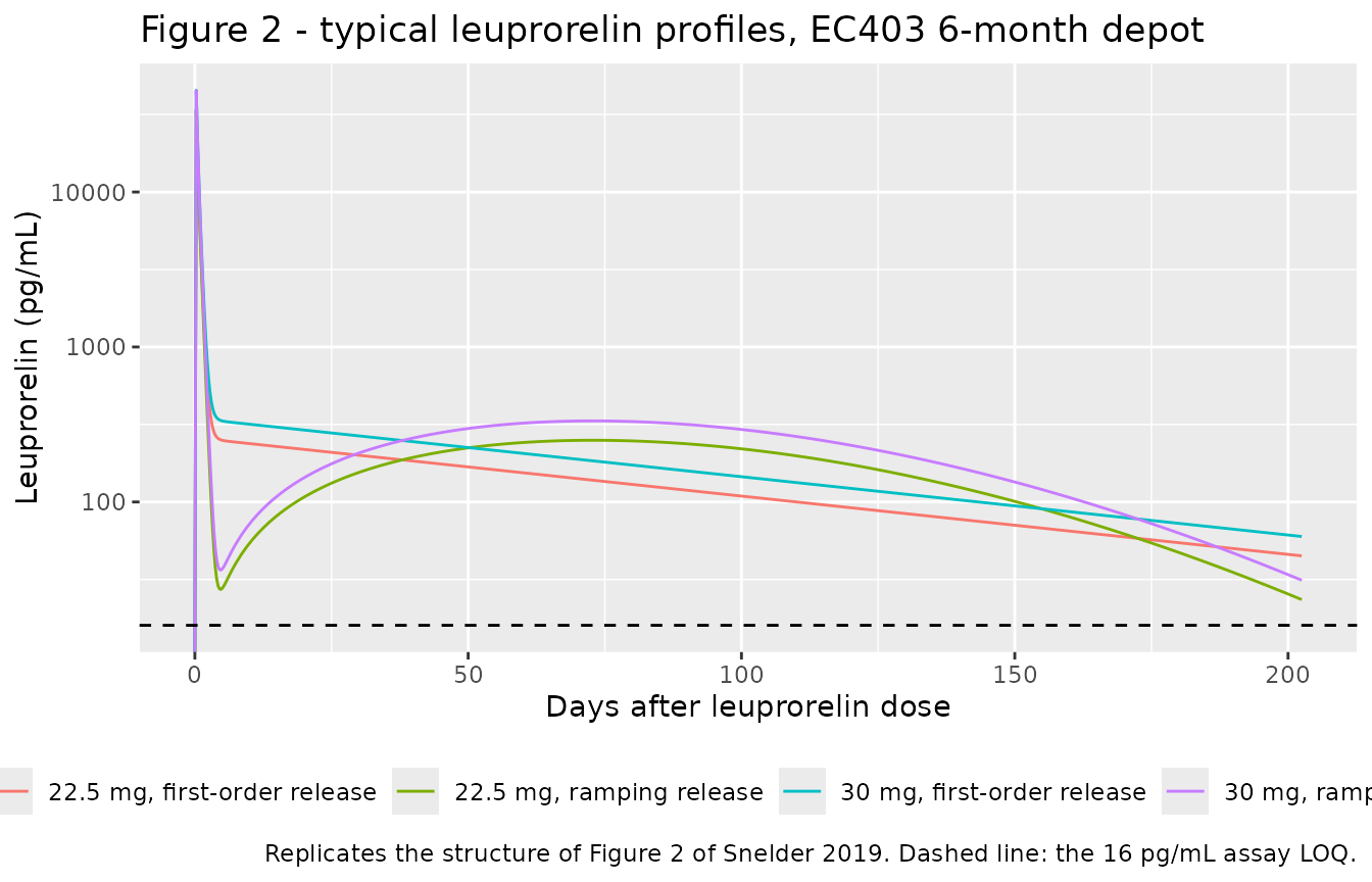
# Replicates Figure 3 of Snelder 2019: the three phases of the testosterone
# response. Phase boundaries are drawn at the leuprorelin dose (day 0) and at
# the end of the assumed CPA effect (day 7).
sim_tv |>
  ggplot(aes(day, TT, colour = arm)) +
  geom_vline(xintercept = c(-7, 0, 7), linetype = "dotted") +
  geom_hline(yintercept = c(50, 20), linetype = "dashed") +
  geom_line() +
  coord_cartesian(xlim = c(-7, 60)) +
  labs(
    x = "Days after leuprorelin dose", y = "Testosterone (ng/dL)",
    colour = NULL,
    title = "Figure 3 - CPA decrease, agonist flare, downregulation suppression",
    caption = paste(
      "Replicates the structure of Figure 3 of Snelder 2019.",
      "Dotted lines: CPA window opens (day -7), leuprorelin dose (day 0),",
      "assumed end of the CPA effect (day 7).",
      "Dashed lines: the 50 and 20 ng/dL castration targets discussed in",
      "Section 4."
    )
  ) +
  theme(legend.position = "bottom")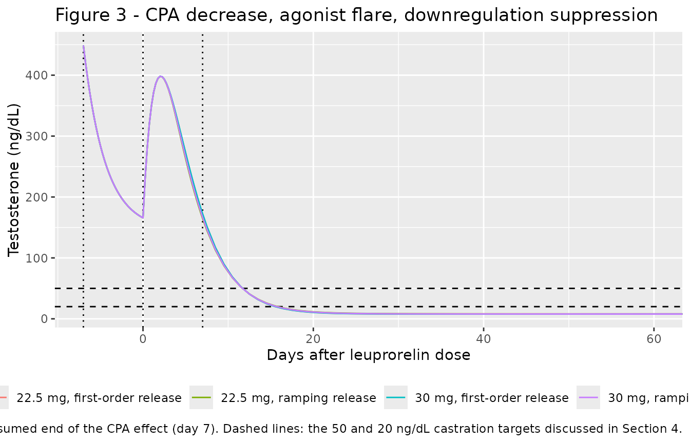
# The three phases are qualitative claims in Results 3.2, so they are checked
# as ordering statements on a deterministic typical-value profile rather than
# against digitised numbers.
phase <- sim_tv |>
  dplyr::group_by(arm) |>
  dplyr::summarise(
    tt_baseline   = TT[which.min(abs(time - 0))],
    tt_predose    = TT[which.min(abs(time - T_DOSE))],
    tt_flare_max  = max(TT[time >= T_DOSE & time <= T_DOSE + 336]),
    tt_nadir      = min(TT[time >= T_DOSE + 28 * 24]),
    psa_baseline  = PSA[which.min(abs(time - 0))],
    psa_final     = PSA[which.max(time)],
    .groups = "drop"
  )

phase |>
  dplyr::rename(
    "Arm" = arm,
    "T at CPA start (ng/dL)" = tt_baseline,
    "T just before leuprorelin (ng/dL)" = tt_predose,
    "Peak T during the flare (ng/dL)" = tt_flare_max,
    "T nadir after day 28 (ng/dL)" = tt_nadir,
    "PSA at CPA start (ng/mL)" = psa_baseline,
    "PSA at day 203 (ng/mL)" = psa_final
  ) |>
knitr::kable(digits = 2, caption = "Typical-value phase summary, EC403.")| Arm | T at CPA start (ng/dL) | T just before leuprorelin (ng/dL) | Peak T during the flare (ng/dL) | T nadir after day 28 (ng/dL) | PSA at CPA start (ng/mL) | PSA at day 203 (ng/mL) |
|---|---|---|---|---|---|---|
| 22.5 mg, first-order release | 449 | 165.73 | 398.09 | 8.00 | 9.73 | 0.49 |
| 22.5 mg, ramping release | 449 | 165.73 | 398.01 | 7.89 | 9.73 | 0.49 |
| 30 mg, first-order release | 449 | 165.73 | 398.21 | 7.88 | 9.73 | 0.49 |
| 30 mg, ramping release | 449 | 165.73 | 398.14 | 7.79 | 9.73 | 0.49 |
stopifnot(
  # Phase 0: the model starts at the published baselines.
  all(abs(phase$tt_baseline - bslt) < 1e-6),
  all(abs(phase$psa_baseline - bslp) < 1e-6),
  # Phase 1: CPA suppresses T before leuprorelin is given.
  all(phase$tt_predose < 0.5 * bslt),
  # Phase 2: the agonist flare pushes T back above its pre-dose value.
  all(phase$tt_flare_max > 1.4 * phase$tt_predose),
  # Phase 3: receptor downregulation drives T below the 50 ng/dL European
  # castration target and below the 20 ng/dL target now being proposed
  # (Discussion, paragraph 1).
  all(phase$tt_nadir < 20),
  # PSA falls toward, and does not undershoot, the closed-form minimum.
  all(phase$psa_final < 0.25 * bslp),
  all(phase$psa_final > 0.98 * psa_min)
)
PSA turnover and the steady-state T-PSA relationship
# Replicates Figure 4 of Snelder 2019: PSA concentrations over the 6-month
# depot interval. The dashed line is the closed-form minimum from Equation 9.
sim_tv |>
  ggplot(aes(day, PSA, colour = arm)) +
  geom_line() +
  geom_hline(yintercept = psa_min, linetype = "dashed") +
  scale_y_log10() +
  labs(
    x = "Days after leuprorelin dose", y = "PSA (ng/mL)", colour = NULL,
    title = "Figure 4 - typical PSA profiles, EC403 6-month depot",
    caption = paste0(
      "Replicates the structure of Figure 4 of Snelder 2019. Dashed line: ",
      "the typical minimal steady-state PSA of ", signif(psa_min, 3),
      " ng/mL implied by Equations 7 and 9."
    )
  ) +
  theme(legend.position = "bottom")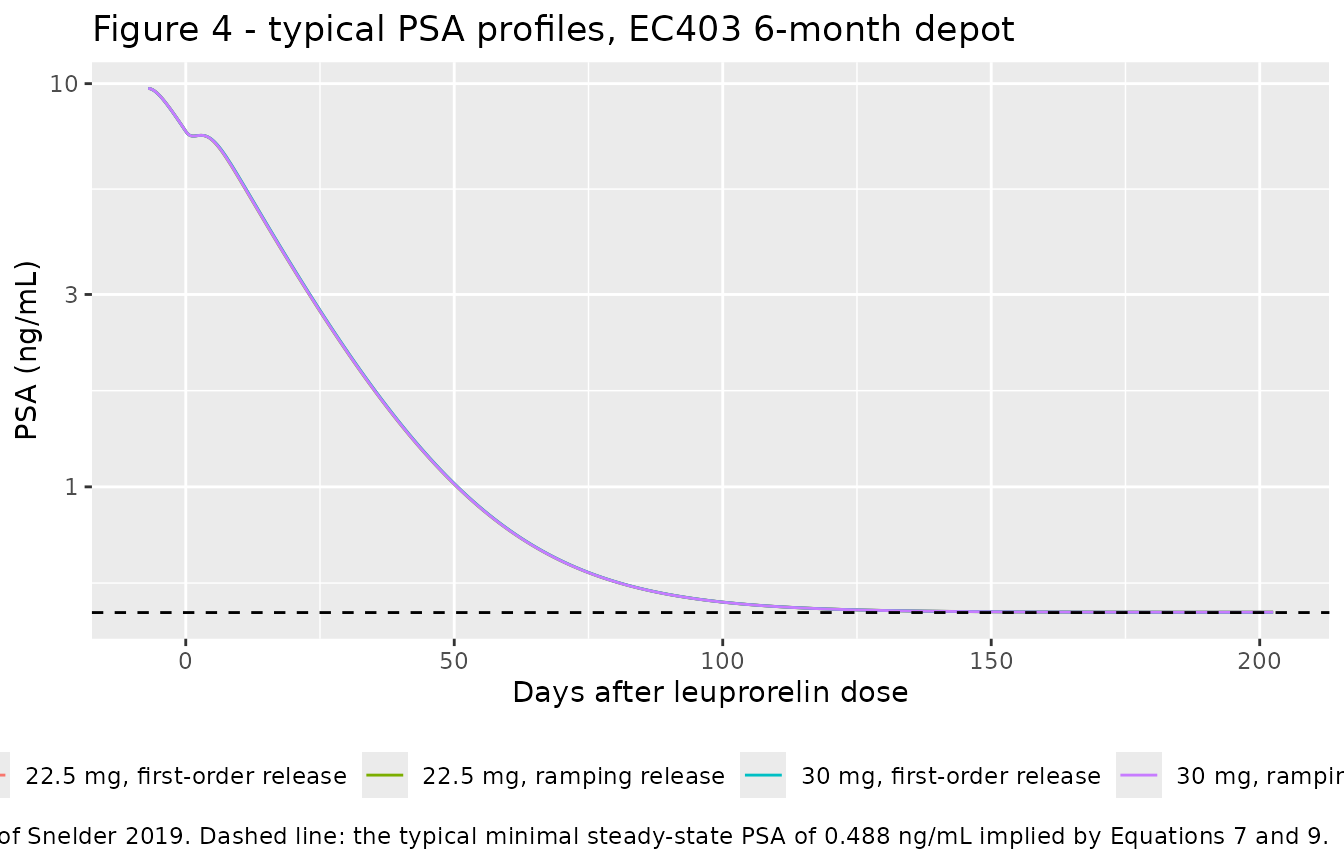
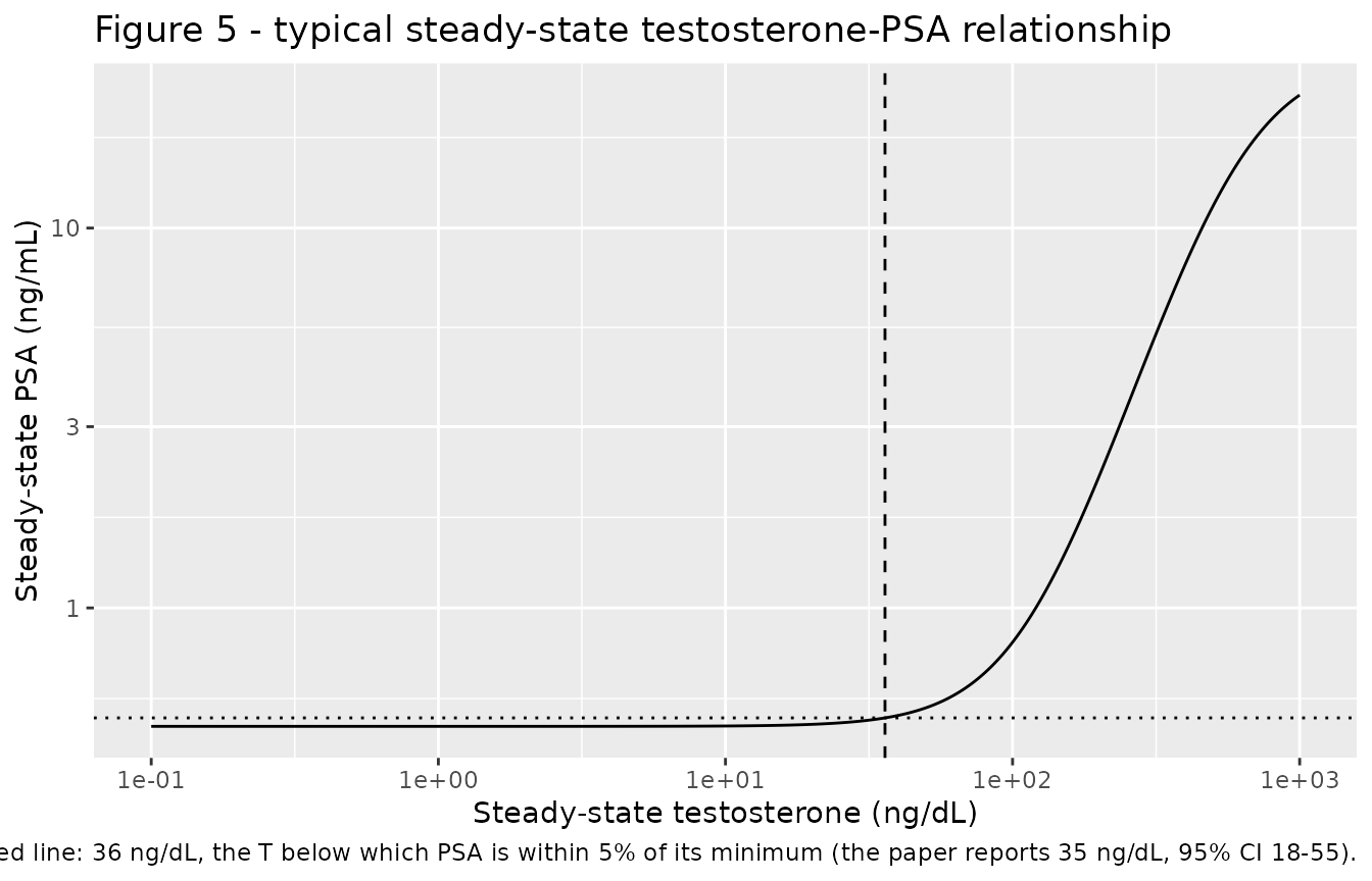
The steady-state relationship of Equation 9 is what the paper’s Figure 5 and its 35 ng/dL conclusion rest on. It is evaluated here directly, and separately confirmed against the simulated PSA the dynamic model settles to at the end of the depot interval.
tt_grid <- 10^seq(log10(0.1), log10(1000), length.out = 400)
ss <- tibble::tibble(
  TT  = tt_grid,
  PSA = psa_min * (1 + eff(tt_grid))
)

ggplot(ss, aes(TT, PSA)) +
  geom_line() +
  geom_vline(xintercept = t_target, linetype = "dashed") +
  geom_hline(yintercept = psa_min / 0.95, linetype = "dotted") +
  scale_x_log10() +
  scale_y_log10() +
  labs(
    x = "Steady-state testosterone (ng/dL)", y = "Steady-state PSA (ng/mL)",
    title = "Figure 5 - typical steady-state testosterone-PSA relationship",
    caption = paste0(
      "Replicates the median curve of Figure 5 of Snelder 2019. Dashed line: ",
      signif(t_target, 3), " ng/dL, the T below which PSA is within 5% of its ",
      "minimum (the paper reports 35 ng/dL, 95% CI 18-55)."
    )
  )
# The dynamic model must land on the algebraic steady-state curve. Both sides
# use the same drawn parameters, so the difference is pure numerical /
# not-quite-steady-state error and a tight bound is correct here.
ss_check <- sim_tv |>
  dplyr::filter(time == max(time)) |>
  dplyr::mutate(psa_closed_form = psa_min * (1 + eff(TT)),
                pct_diff = 100 * (PSA - psa_closed_form) / psa_closed_form)

ss_check |>
  dplyr::select(arm, TT, PSA, psa_closed_form, pct_diff) |>
  dplyr::rename(
    "Arm" = arm, "T at day 203 (ng/dL)" = TT,
    "Simulated PSA (ng/mL)" = PSA,
    "Equation 9 PSA (ng/mL)" = psa_closed_form,
    "Difference (%)" = pct_diff
  ) |>
  knitr::kable(digits = 3,
caption = "Dynamic PSA against the Equation 9 steady state.")| Arm | T at day 203 (ng/dL) | Simulated PSA (ng/mL) | Equation 9 PSA (ng/mL) | Difference (%) |
|---|---|---|---|---|
| 22.5 mg, first-order release | 9.739 | 0.489 | 0.489 | 0.001 |
| 22.5 mg, ramping release | 11.418 | 0.489 | 0.489 | -0.065 |
| 30 mg, first-order release | 9.151 | 0.489 | 0.489 | 0.006 |
| 30 mg, ramping release | 10.363 | 0.489 | 0.489 | -0.036 |
Virtual cohort and variability
The cohort below reproduces the EC403 design: 100 subjects per dose
group, 90% receiving CPA (Results 3.2), and the slow-release phenotype
drawn from the estimated mixture with
P(ramping) = 1 - 0.408 = 0.592 (Table 2 read with Results
3.1).
# set.seed() seeds R's RNG for the covariate draws below. It does NOT seed
# rxode2's simulation RNG, whose streams are partitioned per solver thread, so
# the etas drawn during rxSolve differ between a 2-thread CI runner and a
# 16-thread workstation. Every assertion downstream is written on a centre or a
# robust quantile so that it holds for any cohort the model can produce.
set.seed(20190601)
n_per_arm <- 100L

make_cohort <- function(dose_mg, n, id_offset) {
  tibble::tibble(
    id           = id_offset + seq_len(n),
    dose_mg      = dose_mg,
    cpa_flag     = as.numeric(stats::runif(n) < 0.90),
    MIX_RAMP_REL = as.numeric(stats::runif(n) < 0.592),
    arm          = paste0(dose_mg, " mg")
  )
}

subj_cohort <- dplyr::bind_rows(
  make_cohort(22.5, n_per_arm, 0L),
  make_cohort(30,   n_per_arm, n_per_arm)
)

# A coarser grid than the typical-value one: the cohort is only used for
# variability envelopes, and the render budget is dominated by it.
cohort_grid <- sort(unique(c(seq(0, 336, by = 12), seq(360, 5040, by = 48))))
ev_cohort <- make_ec403_events(subj_cohort, cohort_grid)
stopifnot(!anyDuplicated(unique(ev_cohort[, c("id", "time", "evid", "cmt")])))

sim_cohort <- rxode2::rxSolve(
  mod_6m, ev_cohort, keep = c("arm", "MIX_RAMP_REL")
) |>
  as.data.frame() |>
  collapse_outputs() |>
  dplyr::mutate(day = (time - T_DOSE) / 24)
vpc <- sim_cohort |>
  tidyr::pivot_longer(c(Cc, TT, PSA), names_to = "output", values_to = "value") |>
  dplyr::mutate(output = factor(
    output, levels = c("Cc", "TT", "PSA"),
    labels = c("Leuprorelin (pg/mL)", "Testosterone (ng/dL)", "PSA (ng/mL)")
  )) |>
  dplyr::group_by(output, arm, day) |>
  dplyr::summarise(
    Q05 = stats::quantile(value, 0.05, na.rm = TRUE),
    Q50 = stats::quantile(value, 0.50, na.rm = TRUE),
    Q95 = stats::quantile(value, 0.95, na.rm = TRUE),
    .groups = "drop"
  ) |>
  # Blank, rather than filter out, any quantile that a log axis cannot show.
  # Filtering here would be indistinguishable from a PKNCA input filter to the
  # static vignette lint, and this is only a display concern.
  dplyr::mutate(dplyr::across(c(Q05, Q50, Q95), \(x) na_if_nonpositive(x)))

ggplot(vpc, aes(day, Q50)) +
  geom_ribbon(aes(ymin = Q05, ymax = Q95), alpha = 0.25) +
  geom_line() +
  facet_grid(output ~ arm, scales = "free_y") +
  scale_y_log10() +
  labs(
    x = "Days after leuprorelin dose", y = NULL,
    title = "Median and 90% prediction interval, EC403 virtual cohort",
    caption = paste(
      "Replicates the structure of Figures 2, 3 and 4 of Snelder 2019",
      "(prediction intervals only; the observed data are not public)."
    )
  )
#> Warning: Removed 30 rows containing missing values or values outside the scale range
#> (`geom_ribbon()`).
#> Warning: Removed 30 rows containing missing values or values outside the scale range
#> (`geom_line()`).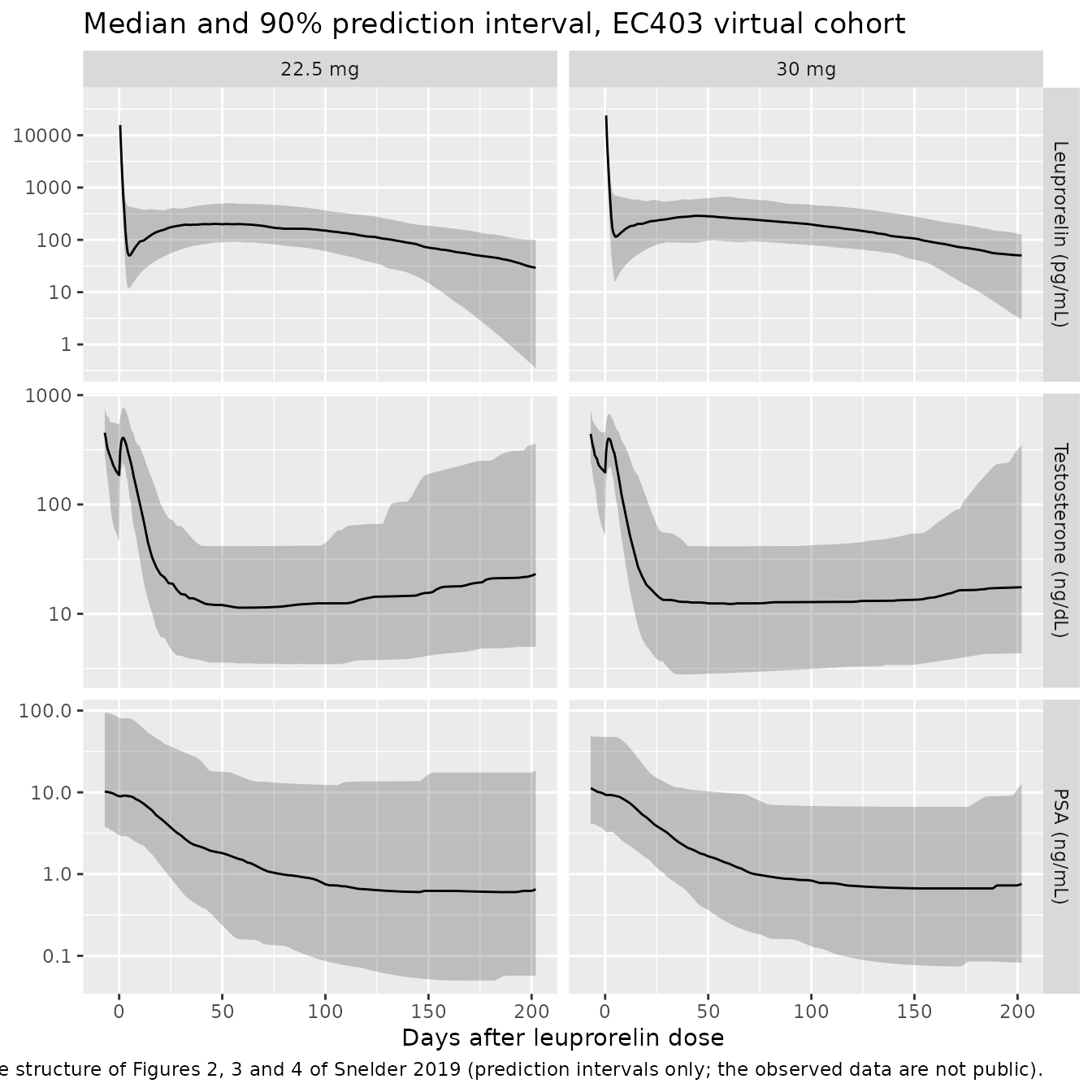
# The paper's cohort-level claims (Results 3.4 / Discussion): the simulated
# minimum PSA has a median of 0.62 ng/mL and, for 90% of patients, lies between
# roughly 0.05 and 10 ng/mL.
psa_min_i <- sim_cohort |>
  dplyr::group_by(id) |>
  dplyr::summarise(psa_min = min(PSA), .groups = "drop")

med_psa_min <- stats::median(psa_min_i$psa_min)
q_psa_min   <- stats::quantile(psa_min_i$psa_min, c(0.05, 0.95))

tibble::tibble(
  Quantity = c("Median minimum PSA (ng/mL)",
               "5th percentile of minimum PSA (ng/mL)",
               "95th percentile of minimum PSA (ng/mL)"),
  Cohort   = c(med_psa_min, q_psa_min[[1]], q_psa_min[[2]]),
  Paper    = c(0.62, 0.05, 10),
  Source   = "Results 3.4 and Discussion paragraph 3"
) |>
  dplyr::mutate(Cohort = signif(Cohort, 3)) |>
knitr::kable(caption = "Cohort minimum-PSA distribution against the paper.")| Quantity | Cohort | Paper | Source |
|---|---|---|---|
| Median minimum PSA (ng/mL) | 0.6060 | 0.62 | Results 3.4 and Discussion paragraph 3 |
| 5th percentile of minimum PSA (ng/mL) | 0.0573 | 0.05 | Results 3.4 and Discussion paragraph 3 |
| 95th percentile of minimum PSA (ng/mL) | 8.9900 | 10.00 | Results 3.4 and Discussion paragraph 3 |
stopifnot(
  # A ratio bound on the centre: a mis-transcribed BSLP, Emax, EC50 or nHP
  # moves the median minimum PSA by tens of percent, while the sampling noise
  # of a 200-subject cohort moves it by a few. Realised 0.54-0.72 across
  # repeated draws at 2 / 4 / 16 threads.
  med_psa_min > 0.62 / 1.6, med_psa_min < 0.62 * 1.6,
  # The paper's "~0.05 to 10 ng/mL for 90% of patients" is a rounded range, so
  # the check is that the cohort's 5-95% span sits inside one order of
  # magnitude of each end rather than matching the endpoints.
  q_psa_min[[1]] > 0.005, q_psa_min[[1]] < 0.5,
  q_psa_min[[2]] > 1,     q_psa_min[[2]] < 100,
  # Every subject must start at the published baselines up to the Box-Cox /
  # log-normal baseline etas, so the cohort medians of the baselines are the
  # right centre check.
  abs(stats::median(sim_cohort$TT[sim_cohort$time == 0]) / bslt - 1) < 0.15,
  abs(stats::median(sim_cohort$PSA[sim_cohort$time == 0]) / bslp - 1) < 0.20
)
PKNCA validation of the leuprorelin PK
Snelder 2019 publishes no non-compartmental analysis of leuprorelin,
so the reference values below are the model’s own exact identities
rather than transcribed table entries. For a typical-value (no-IIV)
solve of a linear disposition model with complete release,
AUC(0-inf) must equal RBIO * Dose / CL, which
is the quantity a mis-transcribed clearance, dose or concentration-unit
conversion breaks immediately.
The NCA solve puts the dose at time = 0 with no
cyproterone acetate, since the drug’s own disposition does not depend on
the PD model.
nca_times <- sort(unique(c(
  seq(0, 24, by = 0.25),        # resolve Tmax of the fast release route
  seq(30, 168, by = 6),
  seq(192, 8760, by = 24)       # one year, the paper's stated validity horizon
)))

subj_nca <- tidyr::crossing(dose_mg = c(22.5, 30), MIX_RAMP_REL = c(0, 1)) |>
  dplyr::mutate(
    id = dplyr::row_number(),
    cpa_flag = 0,
    treatment = paste0(dose_mg, " mg, ",
                       ifelse(MIX_RAMP_REL == 1, "ramping", "first-order"))
  )

ev_nca <- tidyr::crossing(subj_nca, cmt = c("depot", "depot2")) |>
  dplyr::mutate(time = 0, evid = 1L, amt = dose_mg, rate = NA_real_) |>
  dplyr::bind_rows(
    tidyr::crossing(subj_nca, time = nca_times, cmt = ec403_outputs) |>
      dplyr::mutate(evid = 0L, amt = 0, rate = NA_real_)
  ) |>
  dplyr::mutate(CONMED_CYPROTERONE = 0) |>
  dplyr::arrange(id, time, evid) |>
  as.data.frame()

sim_nca_raw <- rxode2::rxSolve(
  tv_6m, ev_nca, keep = c("treatment", "dose_mg")
) |>
  as.data.frame() |>
  collapse_outputs()
#> ℹ omega/sigma items treated as zero: 'etalfdepot', 'etalcl', 'etalogitfrel', 'etalka_slow', 'etaldr50', 'etalkd', 'etalkout_tt', 'etalrbase_tt', 'etalcpa', 'etalhill_dr', 'etalkout_psa', 'etalemax', 'etalec50', 'etalhill_psa', 'etalrbase_psa'
#> Warning: multi-subject simulation without without 'omega'

# Concentrations must be non-negative before PKNCA takes logs on the terminal
# slope; a solver undershoot into the negative tail turns aucinf.obs into NaN.
stopifnot(all(sim_nca_raw$Cc >= -1e-9))

# The PKNCA input filter is `!is.na(Cc)` only: dropping the time-zero row is
# what produces the "AUC range starting (0) before the first measurement"
# warning on every subject.
sim_nca <- sim_nca_raw |>
  dplyr::filter(!is.na(Cc)) |>
  dplyr::mutate(Cc = pmax(Cc, 0)) |>
  dplyr::select(id, time, Cc, treatment)

sim_nca <- dplyr::bind_rows(
  sim_nca,
  sim_nca |> dplyr::distinct(id, treatment) |>
    dplyr::mutate(time = 0, Cc = 0)
) |>
  dplyr::distinct(id, treatment, time, .keep_all = TRUE) |>
  dplyr::arrange(id, treatment, time)

conc_obj <- PKNCA::PKNCAconc(sim_nca, Cc ~ time | treatment + id)

# The event table gives the nominal dose to each depot compartment and lets
# f(depot) / f(depot2) split it, so the administered amount per subject is the
# single nominal dose, not the sum of the two dose records.
dose_df <- ev_nca |>
  dplyr::filter(evid == 1, cmt == "depot") |>
  dplyr::select(id, time, amt, treatment)

dose_obj <- PKNCA::PKNCAdose(dose_df, amt ~ time | treatment + id)

intervals <- data.frame(
  start      = 0,
  end        = Inf,
  cmax       = TRUE,
  tmax       = TRUE,
  auclast    = TRUE,
  aucinf.obs = TRUE,
  half.life  = TRUE
)

nca_res <- PKNCA::pk.nca(
  PKNCA::PKNCAdata(conc_obj, dose_obj, intervals = intervals)
)
cl_6m   <- exp(p6[["lcl"]])
rbio_6m <- exp(p6[["lfdepot"]])

# Reference values. AUC(0-inf) and Cmax are exact model identities; Tmax is the
# closed-form peak time of the fast release route, ln(ka/kel)/(ka - kel), which
# the 0.25 h grid resolves.
ka_fast <- exp(p6[["lka_fast"]])
kel_6m  <- cl_6m / exp(p6[["lvc"]])
tmax_ref <- log(ka_fast / kel_6m) / (ka_fast - kel_6m)

published <- subj_nca |>
  dplyr::transmute(
    treatment,
    # pg/mL * h: Dose (mg) * 1e6 / CL (L/h)
    aucinf.obs = rbio_6m * dose_mg * 1e6 / cl_6m,
    tmax       = tmax_ref
  )

cmp <- nlmixr2lib::ncaComparisonTable(
  simulated = nca_res,
  reference = published,
  by        = "treatment",
  units     = c(aucinf.obs = "pg*h/mL", tmax = "h"),
  tolerance_pct = 20
)

knitr::kable(
  cmp,
  caption = paste(
    "Simulated NCA against the model's exact identities. Snelder 2019",
    "reports no NCA table for leuprorelin; the reference column is",
    "RBIO * Dose / CL for AUC(0-inf) and ln(ka/kel)/(ka - kel) for Tmax.",
    "* differs from reference by >20%."
  )
)| NCA parameter | treatment | Reference | Simulated | % diff |
|---|---|---|---|---|
| Tmax (h) | 22.5 mg, first-order | 1.74 | 1.75 | +0.4% |
| Tmax (h) | 22.5 mg, ramping | 1.74 | 1.75 | +0.4% |
| Tmax (h) | 30 mg, first-order | 1.74 | 1.75 | +0.4% |
| Tmax (h) | 30 mg, ramping | 1.74 | 1.75 | +0.4% |
| AUC0-∞ (obs) (pg*h/mL) | 22.5 mg, first-order | 1290000 | 1290000 | -0.0% |
| AUC0-∞ (obs) (pg*h/mL) | 22.5 mg, ramping | 1290000 | 1290000 | -0.0% |
| AUC0-∞ (obs) (pg*h/mL) | 30 mg, first-order | 1720000 | 1720000 | -0.0% |
| AUC0-∞ (obs) (pg*h/mL) | 30 mg, ramping | 1720000 | 1720000 | -0.0% |
nca_wide <- as.data.frame(nca_res) |>
  dplyr::select(treatment, PPTESTCD, PPORRES) |>
  tidyr::pivot_wider(names_from = PPTESTCD, values_from = PPORRES) |>
  dplyr::left_join(published, by = "treatment",
                   suffix = c("", "_ref"))

stopifnot(
  # Mass balance: every mg released must appear in the AUC. Deterministic, so
  # the bound is set by the trapezoidal error of the sampling grid, not by
  # cohort noise.
  max(abs(nca_wide$aucinf.obs / nca_wide$aucinf.obs_ref - 1)) < 0.02,
  # The peak is the fast route's, so Tmax must sit within one grid step of the
  # closed form.
  max(abs(nca_wide$tmax - tmax_ref)) <= 0.25,
  # The two doses differ only by a scale factor in a linear model.
  {
    r <- nca_wide$aucinf.obs[nca_wide$treatment == "30 mg, ramping"] /
      nca_wide$aucinf.obs[nca_wide$treatment == "22.5 mg, ramping"]
    abs(r - 30 / 22.5) < 0.01
  }
)
The two EC402 formulations
Supplement 1 fits a separate PK model to each EC402 formulation. Both are reproduced here on the repeated-dose schedules the study used: monthly for the 1-month depot and every four months for the 4-month depot, over the eight months of EC402 follow-up shown in Figure S1.2.
# The slow-release depots take a zero-order input of modelled duration
# (dur(depot2) / dur(depot3) in the model files), which requires rate = -2 on
# those dose records.
make_pk_events <- function(dose_mg, dose_times, obs_times,
                           bolus_cmts, infusion_cmts = character()) {
  bolus <- tidyr::crossing(time = dose_times, cmt = bolus_cmts) |>
    dplyr::mutate(evid = 1L, amt = dose_mg, rate = NA_real_)
  inf <- if (length(infusion_cmts)) {
    tidyr::crossing(time = dose_times, cmt = infusion_cmts) |>
      dplyr::mutate(evid = 1L, amt = dose_mg, rate = -2)
  } else NULL
  obs <- tibble::tibble(time = obs_times, cmt = "central",
                        evid = 0L, amt = 0, rate = NA_real_)
  dplyr::bind_rows(bolus, inf, obs) |>
    dplyr::mutate(id = 1L) |>
    dplyr::arrange(time, evid) |>
    as.data.frame()
}

obs_402 <- sort(unique(c(seq(0, 48, by = 0.5), seq(54, 5832, by = 6))))

ev_1m <- make_pk_events(
  dose_mg = 3.75, dose_times = seq(0, 5040, by = 672),
  obs_times = obs_402, bolus_cmts = "depot", infusion_cmts = "depot2"
)
ev_4m <- make_pk_events(
  dose_mg = 15, dose_times = c(0, 2880), obs_times = obs_402,
  bolus_cmts = c("depot", "depot2"), infusion_cmts = "depot3"
)

sim_402 <- dplyr::bind_rows(
  as.data.frame(rxode2::rxSolve(tv_1m, ev_1m)) |>
    dplyr::mutate(formulation = "1-month depot, 3.75 mg"),
  as.data.frame(rxode2::rxSolve(tv_4m, ev_4m)) |>
    dplyr::mutate(formulation = "4-month depot, 15 mg")
) |>
  dplyr::filter(!is.na(Cc))
#> ℹ omega/sigma items treated as zero: 'etalka_slope', 'etalfrel', 'etalfdepot'
#> ℹ omega/sigma items treated as zero: 'etalfdepot', 'etalka_slope', 'etalogitfrel', 'etalogitfrel2'

sim_402 |>
  dplyr::mutate(Cc = na_if_nonpositive(Cc)) |>
  ggplot(aes(time, Cc)) +
  geom_line() +
  geom_hline(yintercept = 16, linetype = "dashed") +
  facet_wrap(~formulation, ncol = 1) +
  scale_y_log10() +
  labs(
    x = "Time (h)", y = "Leuprorelin (pg/mL)",
    title = "Figure S1.2 - typical EC402 profiles",
    caption = paste(
      "Replicates the structure of Figure S1.2 of Snelder 2019 Supplement 1.",
      "Dashed line: the 16 pg/mL assay LOQ."
    )
  )
#> Warning: Removed 2 rows containing missing values or values outside the scale range
#> (`geom_line()`).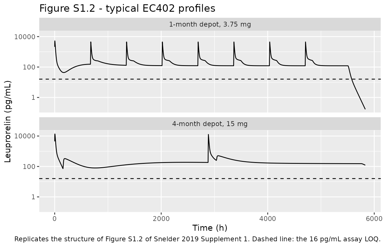
# Dose fractions must partition the dose exactly, and the flat maintenance
# phase must sit above the assay LOQ - the two properties Figure S1.2 shows.
frel_1m  <- exp(theta(ui_1m, "lfrel"))
frel_4m  <- plogis(theta(ui_4m, "logitfrel"))
frel2_4m <- plogis(theta(ui_4m, "logitfrel2"))

fractions <- tibble::tibble(
  Model = c(rep("1-month depot", 2), rep("4-month depot", 3)),
  Route = c("fast", "slow (ramping)",
            "fast", "slow (lagged first-order)", "slow (ramping)"),
  Model_fraction = c(
    frel_1m, 1 - frel_1m,
    frel_4m, (1 - frel_4m) * frel2_4m, (1 - frel_4m) * (1 - frel2_4m)
  ),
  Paper_fraction = c(0.441, 0.559, 0.31, 0.11, 0.58),
  Source = c(rep("Table S1.1 footnote", 2), rep("Table S1.2 footnote", 3))
)

fractions |>
  dplyr::mutate(Model_fraction = signif(Model_fraction, 3)) |>
  dplyr::rename("Model fraction" = Model_fraction,
                "Paper fraction" = Paper_fraction) |>
knitr::kable(caption = "Release-route dose fractions, EC402.")| Model | Route | Model fraction | Paper fraction | Source |
|---|---|---|---|---|
| 1-month depot | fast | 0.441 | 0.441 | Table S1.1 footnote |
| 1-month depot | slow (ramping) | 0.559 | 0.559 | Table S1.1 footnote |
| 4-month depot | fast | 0.310 | 0.310 | Table S1.2 footnote |
| 4-month depot | slow (lagged first-order) | 0.114 | 0.110 | Table S1.2 footnote |
| 4-month depot | slow (ramping) | 0.576 | 0.580 | Table S1.2 footnote |
maint <- sim_402 |>
  dplyr::group_by(formulation) |>
  dplyr::summarise(
    cmax        = max(Cc),
    tmax        = time[which.max(Cc)],
    median_flat = stats::median(Cc[time >= 336 & time <= 5040]),
    .groups = "drop"
  )

maint |>
  dplyr::rename("Formulation" = formulation, "Cmax (pg/mL)" = cmax,
                "Tmax (h)" = tmax,
                "Median day 14-210 (pg/mL)" = median_flat) |>
knitr::kable(digits = 1, caption = "EC402 typical-value profile summary.")| Formulation | Cmax (pg/mL) | Tmax (h) | Median day 14-210 (pg/mL) |
|---|---|---|---|
| 1-month depot, 3.75 mg | 5223.8 | 3 | 133.9 |
| 4-month depot, 15 mg | 13706.5 | 4 | 166.9 |
stopifnot(
  # Fractions partition the dose to the two decimals the footnotes print.
  all(abs(fractions$Model_fraction - fractions$Paper_fraction) < 0.006),
  abs(sum(fractions$Model_fraction[1:2]) - 1) < 1e-12,
  abs(sum(fractions$Model_fraction[3:5]) - 1) < 1e-12,
  # Figure S1.2 shows an initial peak in the 10^3-10^4 pg/mL decade and a
  # maintenance phase in the 10^2 decade, both well above the 16 pg/mL LOQ.
  all(maint$cmax > 300), all(maint$cmax < 3e4),
  all(maint$median_flat > 16), all(maint$median_flat < 1000),
  # The peak belongs to the fast first-order route, so it arrives within the
  # first day.
  all(maint$tmax < 24)
)
Assumptions and deviations
The mixture class is a data column, not a fitted latent variable. rxode2 has no
$MIXTUREconstruct, so the EC403 slow-release phenotype arrives as the covariateMIX_RAMP_RELand the estimated mixture proportion (prop Pop1= 0.408, Table 2) is recorded in the model’scovariateData$MIX_RAMP_REL$notesinstead of inini(), sincemodel()never references it. The cohort above drawsMIX_RAMP_REL ~ Bernoulli(0.592).The two mixture populations are numbered oppositely in the main text and in Supplement 4. Results 3.1 states that “41% and 59% of the subjects were assigned to population 1 (1st-order release) and population 2 (time dependent release), respectively”, whereas the Supplement 4 control stream has
IF (POP .EQ. 1) K34 = SLP * TIME / 1E6, i.e. population 1 ramping. These do not conflict on substance: Supplement 4 is the sequential T-PSA run in which the class arrives as a per-subject data item with numbering local to that run, while Table 2’sprop Pop1comes from the EC403 PK$MIXTURErun. The extraction follows the main text’s explicit and self-consistent mechanism-to-fraction mapping: 40.8% constant first-order, 59.2% ramping.The cyproterone acetate window is supplied as data. Methods 2.5 assumes a two-week CPA effect and Supplement 4 implements it as a 336 h window opening 168 h before the leuprorelin dose. Because the window’s placement is a protocol fact rather than a fitted parameter, it is carried in the time-varying
CONMED_CYPROTERONEcolumn rather than hard-coded inmodel(). Ninety percent of EC403 subjects received CPA (Results 3.2), which the cohort above reproduces.agonist_kd_ratiois fixed to 1 and the potency parameters are conditional on it. The Discussion is explicit that “the model parameters DR50, Kd and nHT of the T model are sensitive to these assumptions. Hence, they should not be used outside the context of the model.”KoutTis not sensitive to them.Supplement 4’s
$OMEGAdisagrees with Table 4 in two places, and Table 4 wins. The control stream prints0.517for the EC50 variance and-0.00743for the KoutP-EC50 covariance. Only Table 4’s0.0517and-0.00734reproduce the correlation column that Table 4 itself prints (0.375 and -0.0834);0.517would give a correlation of 0.119. Both Table 4 values are used.Table 4’s CV% for the PSA baseline is misprinted. The row reads “omega^2 BSLPSA (CV%) 0.780 (10.9%)”, but the paper’s own CV formula,
sqrt(exp(omega^2) - 1) * 100, gives 108.7% for a variance of 0.780. The variance is used; the CV% is not.No IIV on clearance is carried in the 1-month EC402 model. Supplement 1 states that “IIV was identified on RBIO, Ka3_SLP, CL and Fr”, but Table S1.1 reports no
omega^2 CLrow, so the value is not recoverable from any available source. The eta is omitted rather than invented; do not read its absence as evidence that the published model had none.The RBIO-Ka3_SLP covariance in the 1-month model is taken as zero. Table S1.1 reports the Ka3_SLP-Fr and Fr-RBIO covariances but not the third. Zero is used, which reproduces both printed correlations exactly and leaves the 3x3 block positive definite.
Ka3_SLP * TIMEis read as time after the first dose. Supplement 4’s$DESusesTAD1for the EC403 single-dose model, and Figure S1.1 labels the EC402 release arrowsKa3_SLP*TIME. Both are encoded asmax(0, tafd()), so the ramp continues across doses in the repeated-dose EC402 models. The alternative reading (time since the most recent dose) is not supported by any of the available code.The Fr random effect is on the natural scale in the 1-month model only. Table S1.1’s footnote restates 0.441 as a fraction, and its confidence interval is a fraction interval, whereas Table 2 and Table S1.2 back-transform their
Frvalues throughexpit. Methods 2.8 states that random effects were exponential, so the 1-month model useslfrelwith a log-normal eta while the other two uselogitfrelwith a logit-scale eta.Multi-endpoint observation rows carry
cmt = "Cc". The EC403 model has three endpoints, so rxode2 requires each observation row to name its DV compartment.TTandPSAare genuine ODE states;Ccis an algebraic observable, for which rxode2 appends a compartment slot after all seven ODE states (depot,depot2,central,peripheral1,RT,TT,PSA, thenCc). No ODE state is renumbered, so the usual hazard of naming an observable incmtdoes not arise here.No published NCA to compare against. Snelder 2019 reports visual predictive checks rather than a non-compartmental table for leuprorelin, so the PKNCA section is validated against the model’s own exact identities (
RBIO * Dose / CLand the closed-form Tmax of the fast release route) instead of transcribed values.Study EC404 contributes no separate model. Supplement 2 states that EC404’s PK “was predicted by the EC403 PK model assuming linear PK”, and for its 1-month arm by the Study EC401 model, so no new parameters are reported and no fourth model file exists.
Observed data are not public. All figures show model predictions only.