Quinine nanocapsules in Plasmodium berghei-infected rodents (Maciel 2024)
Source:vignettes/articles/Maciel_2024_quinine.Rmd
Maciel_2024_quinine.RmdModel and source
Maciel 2024 built two linked models for quinine given as the free drug or in two lipid-core nanocapsules: NCP80 (poly(epsilon-caprolactone) coated with polysorbate 80, anionic surface) and NCEUD (Eudragit RS100, cationic surface).
-
Maciel_2024_quinine_rat– a two-compartment population PK model of quinine in whole blood of infected rats after a 20 mg/kg IV bolus. -
Maciel_2024_quinine_mouse– the rat PK translated to mice by allometry, driving a parasitemia model (logistic growth minus Emax killing) fitted to the Peters four-day suppressive test.
- Citation: Maciel TR, Funguetto-Ribeiro AC, Olivo LB, Teixeira FEG, Pacheco CO, de Araujo BV, Haas SE. (2024). Improved Malaria Therapy with Cationic Nanocapsules Demonstrated in Plasmodium berghei-Infected Rodents Using Whole Blood Surrogate Population PK/PD Modeling. Pharmaceutics 16(11):1369. doi:10.3390/pharmaceutics16111369.
- Rat model: Preclinical (rat, male Wistar infected with Plasmodium berghei). Two-compartment population PK model for quinine in WHOLE BLOOD after a single 20 mg/kg IV bolus of free quinine or of quinine-loaded polymeric nanocapsules coated with polysorbate 80 (NCP80, anionic) or prepared with Eudragit RS100 (NCEUD, cationic). Nanoencapsulation (either coating) lowers clearance and central volume; the peripheral volume is formulation-specific. Parameters are per kg body weight. See modellib(‘Maciel_2024_quinine_mouse’) for the rat-to-mouse allometric translation and the parasitemia PK/PD model built on it.
- Mouse model: Preclinical (mouse, Plasmodium berghei-infected). Population PK/PD model for quinine given as free drug or as polysorbate-80-coated (NCP80) or Eudragit RS100 (NCEUD) nanocapsules in the Peters four-day suppressive test. The whole-blood PK is a two-compartment model translated from rats by allometry (Table 2 power equations in body weight, with additive nanocapsule shifts on CL, V1 and V2) and carries no between-animal variability; the doses enter the central compartment with complete bioavailability. Percent parasitemia grows logistically towards a fixed ceiling and is killed by an Emax function of the whole-blood concentration, with a formulation-specific Emax. See modellib(‘Maciel_2024_quinine_rat’) for the rat whole-blood popPK model the translation starts from.
- Article: https://doi.org/10.3390/pharmaceutics16111369
- Data source for both models: Michels 2019, https://doi.org/10.2147/IJN.S227914
Population
Rats. Eighteen male Wistar rats infected with P. berghei received a single 20 mg/kg quinine IV bolus on day 7 after infection, six per formulation (free, NCP80, NCEUD). The whole-blood concentrations (197 observations, 0.083-24 h) were not measured: the authors multiplied the plasma concentrations of Michels 2019 by in-vitro erythrocyte partition coefficients of 3.74 (free), 8.92 (NCP80) and 6.48 (NCEUD) (Methods 2.1-2.2, Results 3.1-3.2). Body weights are not reported.
Mice. Four groups of five P. berghei-infected mice (free quinine, NCP80, NCEUD, saline) were infected on day 0 and dosed 20 mg/kg twice daily intraperitoneally from day 0.5 to day 3.5; 147 parasitemia readings were modelled (Methods 2.1 and 2.4, Results 3.4). No quinine was measured in the mice. The PD model was fitted against whole-blood profiles simulated from the allometric PK (Figure 5).
str(readModelDb("Maciel_2024_quinine_rat")()$population)
#> List of 9
#>  $ species       : chr "rat (male Wistar, Plasmodium berghei-infected)"
#>  $ n_subjects    : int 18
#>  $ n_studies     : int 1
#>  $ weight_range  : chr "(not reported)"
#>  $ sex_female_pct: num 0
#>  $ disease_state : chr "Plasmodium berghei malaria; PK studied on day 7 after infection. The erythrocyte partition coefficients were me"| __truncated__
#>  $ dose_range    : chr "Single 20 mg/kg quinine IV bolus as free quinine, NCP80 or NCEUD (n = 6 per group)"
#>  $ regions       : chr "Brazil (Federal University of Pampa)"
#>  $ notes         : chr "197 whole-blood concentrations sampled at 0.083-24 h (Results 3.2). The whole-blood values were not measured di"| __truncated__
str(readModelDb("Maciel_2024_quinine_mouse")()$population)
#> List of 8
#>  $ species      : chr "mouse (Plasmodium berghei-infected; strain not reported)"
#>  $ n_subjects   : int 20
#>  $ n_studies    : int 1
#>  $ weight_range : chr "(not reported)"
#>  $ disease_state: chr "Plasmodium berghei malaria, Peters four-day suppressive test: infection on day 0 (inoculum 1e8 infected erythro"| __truncated__
#>  $ dose_range   : chr "Quinine 20 mg/kg twice daily intraperitoneally from day 0.5 to day 3.5, as free quinine, NCP80 or NCEUD; saline controls"
#>  $ regions      : chr "Brazil (Federal University of Pampa)"
#>  $ notes        : chr "Four groups of five mice (free quinine, NCP80, NCEUD, saline); 147 parasitemia observations (Results 3.4). The "| __truncated__
Source trace
| Parameter / equation | Value | Source location |
|---|---|---|
| Rat: two-compartment ODEs | n/a | Equations 2-4 |
Rat lcl_free, lcl_nc
|
0.156, 0.059 L/h/kg | Table 1 (CL_pop, CL_NC) |
Rat lvc_free, lvc_nc
|
0.261, 0.028 L/kg | Table 1 (V1_pop, V1_NC) |
Rat lq
|
0.025 L/h/kg | Table 1 (Q_pop) |
Rat lvp_free, lvp_ncp80,
lvp_nceud
|
0.066, 0.204, 0.099 L/kg | Table 1 (V2_pop, V2_NCP80, V2_NCEUD) |
| Rat IIV CL, V1, Q, V2 | 8.5, 1.3, 89.8, 184.4 % CV | Table 1, IIV column |
Rat propSd
|
0.436 | Table 1, proportional model 43.6 |
Mouse allometry lcl, e_wt_cl
|
0.0112, -1.43 | Table 2, CL_SPECIE |
Mouse allometry lvc, e_wt_vc
|
0.00227, -2.06 | Table 2, V1_SPECIE |
Mouse allometry lvp, e_wt_vp
|
0.031, -1.22 | Table 2, V2_SPECIE |
Mouse allometry lq, e_wt_q
|
0.0136, -1.93 | Table 2, Q_SPECIE |
Mouse e_form_nc_cl, e_form_nc_vc
|
-1.353, -3.695 | Table 2, influence of nanostructures in mice |
Mouse e_form_ncp80_vp,
e_form_nceud_vp
|
+4.494, +0.274 | Table 2, influence of nanostructures in mice |
| Mouse PD ODE | n/a | Equation 5 |
Mouse lkg
|
0.012 1/h | Table 3, kg_pop |
Mouse lnmax
|
9.2 % (fixed) | Table 3, Nmax |
Mouse lemax_free, lemax_ncp80,
lemax_nceud
|
0.055, 0.025, 0.069 1/h | Table 3, Results 3.4 |
Mouse lec50
|
3.59 mg/L | Table 3, EC50_pop |
| Mouse IIV Emax, EC50 | 0.008, 5.9 % CV | Table 3, IIV column |
Mouse addSd, propSd
|
0.933 %, 0.0934 | Table 3, residual variability |
Mouse lrbase (initial parasitemia) |
2.0 % (fixed) | Not reported; derived from Figure 6a (see Assumptions) |
The rat column of Table 2 restates Table 1 as additive shifts, which the packaged values reproduce:
t1 <- c(cl_free = 0.156, cl_nc = 0.059, vc_free = 0.261, vc_nc = 0.028,
        vp_free = 0.066, vp_ncp80 = 0.204, vp_nceud = 0.099)
t2_shift <- c(
  cl_nc = t1[["cl_free"]] - 0.0973, vc_nc = t1[["vc_free"]] - 0.233,
  vp_ncp80 = t1[["vp_free"]] + 0.138, vp_nceud = t1[["vp_free"]] + 0.0335
)
pct <- 100 * (t2_shift / t1[names(t2_shift)] - 1)
round(pct, 1)
#>    cl_nc    vc_nc vp_ncp80 vp_nceud
#>     -0.5      0.0      0.0      0.5
# Each Table 2 shift lands within 1% of the Table 1 value (rounding only).
stopifnot(all(abs(pct) < 1))
Rat whole-blood PK
Virtual cohort and simulation
mod_rat <- readModelDb("Maciel_2024_quinine_rat")

forms <- tibble::tibble(
  formulation = c("Free QN", "NCP80", "NCEUD"),
  FORM_QUININE_NCP80 = c(0, 1, 0),
  FORM_QUININE_NCEUD = c(0, 0, 1)
)

n_per_arm <- 100
obs_times <- sort(unique(c(seq(0, 2, by = 0.083), seq(2.25, 24, by = 0.25),
                           seq(25, 96, by = 1))))

make_rat_arm <- function(i) {
  f <- forms[i, ]
  ids <- (i - 1) * n_per_arm + seq_len(n_per_arm)
  dose <- tibble::tibble(id = ids, time = 0, amt = 20, evid = 1, cmt = "central")
  obs <- tidyr::expand_grid(id = ids, time = obs_times) |>
    dplyr::mutate(amt = 0, evid = 0, cmt = "central")
  dplyr::bind_rows(dose, obs) |>
    dplyr::mutate(
      formulation = f$formulation,
      FORM_QUININE_NCP80 = f$FORM_QUININE_NCP80,
      FORM_QUININE_NCEUD = f$FORM_QUININE_NCEUD
    )
}
ev_rat <- dplyr::bind_rows(lapply(seq_len(nrow(forms)), make_rat_arm)) |>
  dplyr::arrange(id, time, dplyr::desc(evid))
stopifnot(!anyDuplicated(unique(ev_rat[, c("id", "time", "evid")])))

rxode2::rxSetSeed(20241125)
sim_rat <- rxode2::rxSolve(mod_rat, events = ev_rat, keep = "formulation") |>
  as.data.frame()
#> ℹ parameter labels from comments will be replaced by 'label()'
Figure 3a – VPC by formulation
sim_rat |>
  dplyr::filter(time > 0, time <= 25) |>
  dplyr::group_by(formulation, time) |>
  dplyr::summarise(
    Q10 = quantile(Cc, 0.10), Q50 = median(Cc), Q90 = quantile(Cc, 0.90),
    .groups = "drop"
  ) |>
  dplyr::mutate(formulation = factor(formulation, levels = forms$formulation)) |>
  ggplot(aes(time, Q50)) +
  geom_ribbon(aes(ymin = Q10, ymax = Q90), alpha = 0.25) +
  geom_line() +
  facet_wrap(~formulation) +
  scale_y_log10() +
  labs(
    x = "Time (h)", y = "Whole-blood quinine (mg/L)",
    caption = "Replicates Figure 3a of Maciel 2024: median and 10th-90th percentiles."
  )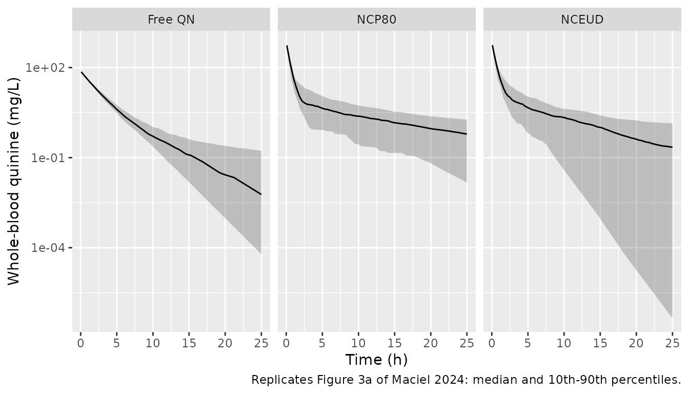
The simulated medians start near 100 mg/L for free quinine and 400-700 mg/L for the nanocapsules and fall to about 1 mg/L by 8 h (free) and below 1 mg/L by 24 h (nanocapsules), as in the published VPC.
PKNCA validation
The paper reports the mean whole-blood AUC0-inf of the data (Results 3.1).
# The ODE solve undershoots zero by about atol in the far tail; assert that it
# is only noise, floor it, and drop the numerically-zero tail so the
# half-life fit does not follow integrator noise.
stopifnot(all(sim_rat$Cc >= -1e-6 * max(sim_rat$Cc, na.rm = TRUE), na.rm = TRUE))
conc_rat <- sim_rat |>
  dplyr::filter(!is.na(Cc)) |>
  dplyr::mutate(Cc = pmax(Cc, 0)) |>
  dplyr::group_by(id) |>
  dplyr::filter(time <= time[which.max(Cc)] | Cc >= 1e-6 * max(Cc)) |>
  dplyr::ungroup() |>
  dplyr::select(id, time, Cc, formulation)
dose_rat <- ev_rat |>
  dplyr::filter(evid == 1) |>
  dplyr::select(id, time, amt, formulation)

nca_rat <- PKNCA::pk.nca(PKNCA::PKNCAdata(
  PKNCA::PKNCAconc(conc_rat, Cc ~ time | formulation + id),
  PKNCA::PKNCAdose(dose_rat, amt ~ time | formulation + id, route = "intravascular"),
  intervals = data.frame(start = 0, end = Inf, cmax = TRUE, aucinf.obs = TRUE, half.life = TRUE)
))

published_rat <- tibble::tribble(
  ~formulation, ~aucinf.obs,
  "Free QN",    127.8,
  "NCP80",      330.9,
  "NCEUD",      397.9
)

cmp_rat <- nlmixr2lib::ncaComparisonTable(
  simulated = nca_rat,
  reference = published_rat,
  by = "formulation",
  units = c(aucinf.obs = "mg*h/L"),
  tolerance_pct = 20
)
knitr::kable(cmp_rat, caption = "Simulated median vs. published mean whole-blood AUC0-inf. * differs by >20%.")| NCA parameter | formulation | Reference | Simulated | % diff |
|---|---|---|---|---|
| AUC0-∞ (obs) (mg*h/L) | Free QN | 128 | 127 | -0.3% |
| AUC0-∞ (obs) (mg*h/L) | NCP80 | 331 | 335 | +1.4% |
| AUC0-∞ (obs) (mg*h/L) | NCEUD | 398 | 338 | -15.1% |
auc_med <- as.data.frame(nca_rat) |>
  dplyr::filter(PPTESTCD == "aucinf.obs") |>
  dplyr::group_by(formulation) |>
  dplyr::summarise(auc = median(PPORRES), .groups = "drop") |>
  dplyr::left_join(published_rat, by = "formulation") |>
  dplyr::mutate(pct = 100 * (auc / aucinf.obs - 1))
auc_med
#> # A tibble: 3 × 4
#>   formulation   auc aucinf.obs     pct
#>   <chr>       <dbl>      <dbl>   <dbl>
#> 1 Free QN      127.       128.  -0.333
#> 2 NCEUD        338.       398. -15.1
#> 3 NCP80        335.       331.   1.37
# AUC = dose / CL, and CL carries only 8.5% CV, so the cohort median sits
# within a few percent of 20 / CL_typical = 128 (free) and 339 (either
# nanocapsule). The NCEUD data mean (397.9) is about 15% above that because
# Table 1 gives both nanocapsules the same clearance.
stopifnot(all(abs(auc_med$pct) < 20))
Mouse PK/PD
Mouse PK at 25 g
The mouse weight is not reported. The vignette uses 0.025 kg, which the paper’s own numbers support: Maciel 2024 (Discussion) quotes a mouse whole-blood AUC0-inf of 36.6 mgh/L for free quinine at 80 mg/kg from Pussard 2003, the data the allometry was fitted to, and the Table 2 clearance at 0.025 kg gives 80 / 2.19 = 36.6 mgh/L.
mod_mouse <- readModelDb("Maciel_2024_quinine_mouse")
mod_mouse_typ <- rxode2::zeroRe(mod_mouse)
#> ℹ parameter labels from comments will be replaced by 'label()'

ev_pussard <- dplyr::bind_rows(
  tibble::tibble(id = 1L, time = 0, amt = 80, evid = 1, cmt = "central"),
  tibble::tibble(id = 1L, time = sort(unique(c(seq(0, 2, 0.05), seq(2.5, 72, 0.5)))),
                 amt = 0, evid = 0, cmt = "central")
) |>
  dplyr::mutate(WT = 0.025, FORM_QUININE_NCP80 = 0, FORM_QUININE_NCEUD = 0,
                treatment = "Free QN 80 mg/kg")
# A one-subject solve returns no id column; PKNCA needs one.
sim_pussard <- rxode2::rxSolve(mod_mouse_typ, events = ev_pussard, keep = "treatment") |>
  as.data.frame() |>
  dplyr::mutate(id = 1L)
#> ℹ omega/sigma items treated as zero: 'etalemax', 'etalec50'

nca_mouse <- PKNCA::pk.nca(PKNCA::PKNCAdata(
  PKNCA::PKNCAconc(dplyr::filter(sim_pussard, !is.na(Cc)), Cc ~ time | treatment + id),
  PKNCA::PKNCAdose(dplyr::filter(ev_pussard, evid == 1), amt ~ time | treatment + id,
                   route = "intravascular"),
  intervals = data.frame(start = 0, end = Inf, aucinf.obs = TRUE)
))
cmp_mouse <- nlmixr2lib::ncaComparisonTable(
  simulated = nca_mouse,
  reference = tibble::tibble(treatment = "Free QN 80 mg/kg", aucinf.obs = 36.6),
  by = "treatment",
  units = c(aucinf.obs = "mg*h/L"),
  tolerance_pct = 20
)
knitr::kable(cmp_mouse, caption = "Typical mouse (25 g) whole-blood AUC0-inf vs. the Pussard 2003 value quoted by Maciel 2024.")| NCA parameter | treatment | Reference | Simulated | % diff |
|---|---|---|---|---|
| AUC0-∞ (obs) (mg*h/L) | Free QN 80 mg/kg | 36.6 | 36.6 | -0.1% |
auc_pussard <- as.data.frame(nca_mouse)$PPORRES[as.data.frame(nca_mouse)$PPTESTCD == "aucinf.obs"]
# Deterministic typical-value solve: only trapezoid and integrator error remain.
stopifnot(abs(auc_pussard / 36.6 - 1) < 0.03)
Figure 5 – simulated mouse dosing regimen
dose_times <- seq(12, 84, by = 12)   # day 0.5 to day 3.5, twice daily
pd_times <- sort(unique(round(c(seq(0, 320, by = 1), seq(12, 96, by = 0.1)), 1)))

mouse_arms <- tibble::tibble(
  treatment = c("Free QN", "NCP80", "NCEUD", "Control"),
  FORM_QUININE_NCP80 = c(0, 1, 0, 0),
  FORM_QUININE_NCEUD = c(0, 0, 1, 0),
  dosed = c(TRUE, TRUE, TRUE, FALSE)
)

make_mouse_arm <- function(i, n) {
  a <- mouse_arms[i, ]
  ids <- (i - 1) * n + seq_len(n)
  obs <- tidyr::expand_grid(id = ids, time = pd_times) |>
    dplyr::mutate(amt = 0, evid = 0, cmt = "parasites")
  dose <- if (a$dosed) {
    tidyr::expand_grid(id = ids, time = dose_times) |>
      dplyr::mutate(amt = 20, evid = 1, cmt = "central")
  } else {
    NULL
  }
  dplyr::bind_rows(dose, obs) |>
    dplyr::mutate(
      treatment = a$treatment, WT = 0.025,
      FORM_QUININE_NCP80 = a$FORM_QUININE_NCP80,
      FORM_QUININE_NCEUD = a$FORM_QUININE_NCEUD
    ) |>
    dplyr::arrange(id, time, dplyr::desc(evid))
}

ev_typ <- dplyr::bind_rows(lapply(seq_len(nrow(mouse_arms)), make_mouse_arm, n = 1))
sim_typ <- rxode2::rxSolve(mod_mouse_typ, events = ev_typ, keep = "treatment") |>
  as.data.frame() |>
  dplyr::mutate(treatment = factor(treatment, levels = mouse_arms$treatment))
#> ℹ omega/sigma items treated as zero: 'etalemax', 'etalec50'
#> Warning: multi-subject simulation without without 'omega'

sim_typ |>
  dplyr::filter(treatment != "Control", time >= 4, time <= 150) |>
  ggplot(aes(time, Cc)) +
  geom_line(colour = "red") +
  geom_hline(yintercept = 3.59, linetype = "dashed", colour = "grey50") +
  facet_wrap(~treatment) +
  scale_y_log10(limits = c(0.01, 100)) +
  labs(
    x = "Time (h)", y = "Simulated whole-blood quinine (mg/L)",
    caption = "Replicates Figure 5 of Maciel 2024 (typical mouse, 25 g); dashed line = EC50."
  )
#> Warning in scale_y_log10(limits = c(0.01, 100)): log-10 transformation
#> introduced infinite values.
#> Warning: Removed 91 rows containing missing values or values outside the scale range
#> (`geom_line()`).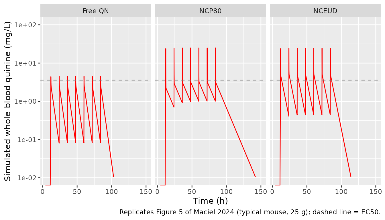
The peaks (about 4.4 mg/L for free quinine and 24 mg/L for both nanocapsules) and troughs fall in the ranges of Figure 5 to within the weight sensitivity described under Assumptions.
Figure 6a – parasitemia by group
rxode2::rxSetSeed(20241126)
ev_vpc <- dplyr::bind_rows(lapply(seq_len(nrow(mouse_arms)), make_mouse_arm, n = 100)) |>
  dplyr::filter(evid == 1 | time %in% seq(0, 320, by = 4))
stopifnot(!anyDuplicated(unique(ev_vpc[, c("id", "time", "evid")])))

sim_vpc <- rxode2::rxSolve(mod_mouse, events = ev_vpc, keep = "treatment") |>
  as.data.frame() |>
  dplyr::mutate(treatment = factor(treatment, levels = mouse_arms$treatment))
#> ℹ parameter labels from comments will be replaced by 'label()'

sim_vpc |>
  dplyr::filter(time >= 24) |>
  dplyr::group_by(treatment, time) |>
  dplyr::summarise(
    Q10 = quantile(sim, 0.10), Q50 = median(sim), Q90 = quantile(sim, 0.90),
    .groups = "drop"
  ) |>
  ggplot(aes(time, Q50)) +
  geom_ribbon(aes(ymin = Q10, ymax = Q90), alpha = 0.25) +
  geom_line() +
  facet_wrap(~treatment) +
  labs(
    x = "Time (h)", y = "Parasitemia (%)",
    caption = "Replicates Figure 6a of Maciel 2024: median and 10th-90th percentiles of simulated observations."
  )
Typical-value check against Figure 6a
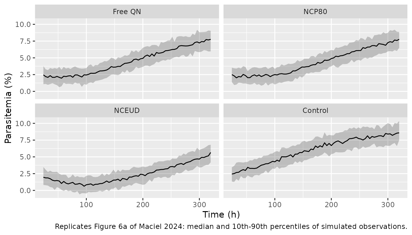
The observed medians below were read from Figure 6a by the maintainers (about +/-0.3 percentage points).
fig6 <- tibble::tribble(
  ~treatment, ~time, ~observed,
  "Control",   24, 2.5,
  "Control",   72, 3.6,
  "Control",  120, 4.9,
  "Control",  168, 6.0,
  "Control",  216, 7.4,
  "Free QN",   24, 2.1,
  "Free QN",   72, 2.1,
  "Free QN",  120, 2.6,
  "Free QN",  168, 3.8,
  "Free QN",  216, 5.0,
  "NCP80",     24, 2.0,
  "NCP80",     72, 2.0,
  "NCP80",    120, 2.5,
  "NCP80",    168, 3.7,
  "NCP80",    216, 5.0,
  "NCEUD",     24, 1.6,
  "NCEUD",     72, 1.0,
  "NCEUD",    120, 1.0,
  "NCEUD",    168, 1.5,
  "NCEUD",    216, 2.4
)
chk6 <- sim_typ |>
  dplyr::filter(time %in% fig6$time) |>
  dplyr::distinct(treatment, time, .keep_all = TRUE) |>
  dplyr::transmute(treatment = as.character(treatment), time, typical = parasites) |>
  dplyr::inner_join(fig6, by = c("treatment", "time")) |>
  dplyr::mutate(diff = typical - observed)
knitr::kable(chk6, digits = 2, caption = "Typical-value parasitemia (%) vs. Figure 6a medians.")| treatment | time | typical | observed | diff |
|---|---|---|---|---|
| Free QN | 24 | 2.26 | 2.1 | 0.16 |
| Free QN | 72 | 2.32 | 2.1 | 0.22 |
| Free QN | 120 | 2.88 | 2.6 | 0.28 |
| Free QN | 168 | 4.11 | 3.8 | 0.31 |
| Free QN | 216 | 5.43 | 5.0 | 0.43 |
| NCP80 | 24 | 2.30 | 2.0 | 0.30 |
| NCP80 | 72 | 2.37 | 2.0 | 0.37 |
| NCP80 | 120 | 2.78 | 2.5 | 0.28 |
| NCP80 | 168 | 3.98 | 3.7 | 0.28 |
| NCP80 | 216 | 5.30 | 5.0 | 0.30 |
| NCEUD | 24 | 1.95 | 1.6 | 0.35 |
| NCEUD | 72 | 1.11 | 1.0 | 0.11 |
| NCEUD | 120 | 1.06 | 1.0 | 0.06 |
| NCEUD | 168 | 1.73 | 1.5 | 0.23 |
| NCEUD | 216 | 2.68 | 2.4 | 0.28 |
| Control | 24 | 2.49 | 2.5 | -0.01 |
| Control | 72 | 3.65 | 3.6 | 0.05 |
| Control | 120 | 4.97 | 4.9 | 0.07 |
| Control | 168 | 6.22 | 6.0 | 0.22 |
| Control | 216 | 7.25 | 7.4 | -0.15 |
stopifnot(
  nrow(chk6) == nrow(fig6),
  # Deterministic solve against a hand-digitised figure: the largest gap is
  # 0.43 percentage points; the digitising error is about 0.3.
  all(abs(chk6$diff) < 0.6),
  # NCEUD is the only arm that pushes parasitemia below its starting level
  # during treatment (Results 3.4).
  chk6$typical[chk6$treatment == "NCEUD" & chk6$time == 120] <
    chk6$typical[chk6$treatment == "Free QN" & chk6$time == 120] - 1
)
Assumptions and deviations
- Rat units. Table 1 labels CL and Q “mL/h” and the volumes “mL”. The values are per kg, in L/h/kg and L/kg, with the dose entered as 20 mg/kg: 20 / 0.156 = 128 mgh/L reproduces the reported free-quinine whole-blood AUC0-inf of 127.8 ugh/mL, and 20 / 0.059 = 339 mg*h/L the nanocapsule values of 330.9 and 397.9.
- Whole-blood data are derived. The rat “whole-blood” concentrations are plasma concentrations times an in-vitro erythrocyte partition coefficient (Methods 2.2), so the model inherits the assumption that Kp is constant over time and concentration.
- Rat IIV. Each entry of the Table 1 IIV column is read as CV% with its RSE in brackets (for example CL “8.5 (32.4)”), the same “value (RSE)” layout as the estimate column. Exponential IIV, OMEGA = log(CV^2 + 1). The reverse reading (RSE first, CV in brackets: CL 32.4%, V1 120.1%, Q 30.0%, V2 29.3%) was considered. It is less consistent with the reported eta-shrinkage: the low shrinkage on Q (6.9%) and V2 (12.8%) needs the large Q and V2 variances of the adopted reading. Under the adopted reading the simulated 24 h medians for the nanocapsules (about 0.5 mg/L NCP80, 0.2 mg/L NCEUD) sit somewhat below the observed medians in Figure 3a (about 0.9 and 0.4 mg/L), and the NCEUD 10th percentile falls far below the plotted range by 24 h, because a small-V2 animal loses the slow phase entirely. Typical-value predictions do not depend on this choice.
- Mouse Emax per formulation. Table 3 lists Emax_pop, Emax_NCP80 and Emax_NCEUD. Results 3.4 describes them as formulation values (“from 0.055 to 0.025 and 0.069”), and the maintainers checked the alternative reading (increments on 0.055): it drives NCP80 parasitemia to about 0.8% by 72 h, whereas Figure 6a shows it flat near 2%. The formulation-value reading reproduces every arm of Figure 6a (table above).
-
Mouse IIV. Table 3 prints the Emax IIV as “0.008”
in the CV% column with no RSE; it is taken as 0.008% CV (effectively
none). Reading it as a variance of 0.008 (about 9% CV) changes the VPC
only marginally. The EC50 IIV is 5.9%
- Mouse residual error. Table 3 prints the additive error as -0.933 with unit “mg/L”. The observation is percent parasitemia and a NONMEM SD estimated as a THETA enters squared, so the model uses an additive SD of 0.933 percentage points.
- Initial parasitemia (non-paper value). The parasite count at infection (N0) is not reported in percent-parasitemia units. The maintainers digitised the saline-control median at the first reading (2.5% at 24 h, Figure 6a) and back-projected it to t = 0 through the reported logistic growth (kg = 0.012 1/h, Nmax = 9.2%), giving 2.0%. With that value the model also reproduces the control medians at 72-216 h.
- Mouse weight (non-paper value). No weight is reported; the vignette uses 0.025 kg, the weight at which the Table 2 clearance reproduces the 36.6 mg*h/L AUC the paper quotes for the Pussard 2003 mouse data. The allometry is steep (exponents -1.22 to -2.06) and the nanocapsule shifts are constants, so predictions are very weight-sensitive: at 0.026 kg the nanocapsule peaks are about 41 mg/L instead of 24, closer to the roughly 45 mg/L of Figure 5, and above 0.0276 kg the nanocapsule central volume becomes negative. Keep WT near 0.025 kg.
- Mouse dosing. Doses are intraperitoneal; with F = 1 assumed (Methods 2.3) and no absorption rate reported, and Figure 5 showing instantaneous peaks, doses enter the central compartment directly. The regimen is seven doses at 12-84 h (day 0.5 to 3.5). Figure 5 also shows a non-zero concentration before the first dose, as if a dose had been given at t = 0; adding it changes the Figure 6a arms by at most 0.5 percentage points, and the protocol in the text is followed.
-
Mouse PK has no variability. The PD was fitted
against a simulated typical profile per formulation (Methods 2.4), so
the mouse PK carries no IIV and no residual error;
Ccis an output, not an endpoint. - Figure 5 troughs. The simulated free-quinine trough (about 0.08 mg/L) is lower than in Figure 5 (about 0.2 mg/L); Figure 5 is drawn on a coarse time grid. Figure 4 (allometric fit to the Pussard data) is not reproduced: its concentration axis sits about 100-fold below the AUC the paper quotes for the same data.
- No erratum or correction notice was found for this article (checked 2026-10-31).