Follitropin delta / FE 999049, multiple dosing with endogenous FSH (Rose 2016b)
Source:vignettes/articles/Rose_2016b_follitropin_delta.Rmd
Rose_2016b_follitropin_delta.RmdModel and source
- Citation: Rose TH, Roshammar D, Erichsen L, Grundemar L, Ottesen JT. Characterisation of Population Pharmacokinetics and Endogenous Follicle-Stimulating Hormone (FSH) Levels After Multiple Dosing of a Recombinant Human FSH (FE 999049) in Healthy Women. Drugs R D. 2016;16(2):165-172. doi:10.1007/s40268-016-0126-z.
- Description: One-compartment population PK model for FE 999049 (recombinant human FSH; INN follitropin delta) after repeated daily subcutaneous dosing in 24 gonadotropin-downregulated healthy women, with first-order absorption through a single transit compartment and first-order elimination. The central compartment holds TOTAL serum FSH: exogenous FE 999049 plus endogenous FSH from a zero-order turnover input that is suppressed over time by observed serum inhibin B through an Imax function. The endogenous FSH baseline decreases with baseline progesterone (power function), and body weight scales CL/F and V/F allometrically (exponents fixed at 0.75 and 1, reference 65 kg).
- Article: https://doi.org/10.1007/s40268-016-0126-z
Rose 2016b characterises the pharmacokinetics of FE 999049 (INN
follitropin delta, a recombinant human FSH expressed in a human cell
line) after seven daily subcutaneous doses of 225 IU. Unlike the
companion single-dose analysis
(Rose_2016_follitropin_delta, doi:10.1007/s40268-016-0129-9), pituitary downregulation
in this trial was incomplete, so measurable endogenous FSH was present
before dosing. The model therefore describes the measured serum FSH as
the sum of exogenous FE 999049 and endogenous FSH (Eq. 4) in one central
compartment:
- dosing site -> transit compartment -> central compartment
(Eqs. 6-7), with first-order elimination
k = CL/F / V/Fshared by both FSH sources; - a zero-order endogenous FSH input
kinthat is suppressed by the observed, time-varying inhibin B level through an Imax function with complete inhibition possible (Eq. 8); - an endogenous FSH baseline
FSHblthat sets the central initial conditionFSHbl * V/Fand decreases with baseline progesterone (power function, Figure 2); -
kinback-calculated per subject from the pre-dose steady state (Section 2.2),kin = k * FSHbl * V/F * (InhB(0) + InhBef) / InhBef.
Population
The FE 999049 arm of a randomised, double-blind, active-controlled multiple-dose trial: 24 healthy women (age 21.5-38.7 years, mean 31.1; weight 46.1-86.6 kg, mean 71.5; BMI 20.8-28.9 kg/m^2) downregulated with a 1-month GnRH-agonist depot on days -28 and -14 (Section 2.1, Table 1). Baseline means were FSH 0.211 ug/L (0.089-0.376), progesterone 0.652 ug/L (0.08-1.49), inhibin B 22.0 pg/mL (4.0-89.0), oestradiol 24.21 pg/mL and LH 0.719 IU/L. Each subject received 225 IU FE 999049 subcutaneously once daily for 7 days. 672 serum FSH samples were collected (pre-dose, daily for 15 days, and every 4 h from the last dose on day 6 to day 8); 3 were below the 0.075 ug/L LLOQ and excluded.
The same information is available programmatically via
readModelDb("Rose_2016b_follitropin_delta")()$meta$population.
Source trace
| Equation / parameter | Value | Source location |
|---|---|---|
lcl (CL/F at 65 kg) |
0.423 L/h | Table 2, row CL/F |
lvc (V/F at 65 kg) |
24.3 L | Table 2, row V/F |
lktr (dosing site -> transit) |
0.329 1/h | Table 2, row ktr |
lka (transit -> central) |
0.148 1/h | Table 2, row ka |
lrbase (FSHbl at progesterone 1 ug/L) |
0.162 ug/L | Table 2, row FSHbl; reference 1 ug/L from the Figure 2 curve |
e_prog_base_rbase |
-0.246 | Table 2, row Progblef |
lec50_inhibinb |
100 pg/mL | Table 2, row InhBef; Section 3 (‘inhibin B concentration giving 50 % inhibition’) |
e_wt_cl, e_wt_vc
|
0.75, 1 (held constant) | Section 3 and Abstract |
etalcl |
15.6% CV -> 0.024045 | Table 2, IIV CV% column |
etalvc |
18.4% CV -> 0.033296 | Table 2, IIV CV% column |
etalktr |
83.4% CV -> 0.52801 | Table 2, IIV CV% column |
etalrbase |
27.8% CV -> 0.074443 | Table 2, IIV CV% column |
addSd, propSd
|
0 (not reported) | Section 3: combined additive + proportional model, magnitudes not published |
d/dt(depot) |
Eq. 6 | Section 3 |
d/dt(transit1) |
Eq. 7 | Section 3 |
d/dt(central) |
Eq. 8 | Section 3 |
central(0) <- rbase * vc |
FSHbl * V/F | Section 2.2 |
kin back-calculation |
pre-dose steady state of Eq. 8 | Section 2.2 |
Allometric scaling (WT/65)^e
|
reference 65 kg | Section 3; Table 2 footnote |
FSHbl * PROG_BASE^Progblef |
un-normalised power function | Section 3; Figure 2 |
IIV variances use omega^2 = log(CV^2 + 1), the same
conversion the companion single-dose model applies to the same authors’
identically formatted Table 2.
Virtual cohort
Covariates are drawn to match Table 1. The paper does not tabulate the inhibin B time course, so each virtual subject carries an illustrative daily inhibin B profile shaped after the purple traces of Figure 5: near baseline for the first days, rising under rFSH stimulation to a peak around day 7 (peaks of a few hundred to about 6000 pg/mL across subjects), and back to baseline by day 12. Inhibin B is a measured model input, not a model prediction, so this profile is a scenario assumption, not a validation target. As in the paper, the daily value is carried forward between samples.
set.seed(2016)
n_sub <- 200L

# Relative inhibin B rise above baseline by study day (illustrative shape
# from Figure 5; 0 = baseline, 1 = individual peak).
inhb_shape <- c(0, 0.02, 0.08, 0.2, 0.4, 0.65, 0.9, 1, 0.75, 0.4, 0.15, 0.05, 0, 0, 0, 0)
inhibinb_at <- function(time_h, base, peak) {
  day <- pmin(floor(time_h / 24), length(inhb_shape) - 1)
  base + peak * inhb_shape[day + 1]
}

rtrunc_lnorm <- function(n, median, sdlog, lo, hi) {
  x <- stats::rlnorm(n, log(median), sdlog)
  pmin(pmax(x, lo), hi)
}

subjects <- tibble::tibble(
  id = seq_len(n_sub),
  WT = pmin(pmax(stats::rnorm(n_sub, 71.5, 9), 46.1), 86.6),
  PROG_BASE = rtrunc_lnorm(n_sub, 0.55, 0.55, 0.08, 1.49),
  INHIBINB_BASE = rtrunc_lnorm(n_sub, 16, 0.75, 4, 89),
  inhb_peak = rtrunc_lnorm(n_sub, 2000, 0.8, 200, 7000)
)

# 225 IU = 13.1 ug, from the specific-activity conversion of the companion
# single-dose paper (Rose 2016, Section 2.2: 37.5/75/150/225/450 IU =
# 2.2/4.4/8.8/13.1/26.3 ug).
dose_ug <- 13.1
dose_times <- seq(0, 144, by = 24)
obs_times <- seq(0, 360, by = 4)

make_events <- function(subj, with_dose = TRUE) {
  obs <- tidyr::expand_grid(id = subj$id, time = obs_times) |>
    dplyr::mutate(evid = 0L, amt = 0, cmt = "central")
  ev <- obs
  if (with_dose) {
    dose <- tidyr::expand_grid(id = subj$id, time = dose_times) |>
      dplyr::mutate(evid = 1L, amt = dose_ug, cmt = "depot")
    ev <- dplyr::bind_rows(dose, obs)
  }
  ev |>
    dplyr::left_join(subj, by = "id") |>
    dplyr::mutate(
      INHIBINB = inhibinb_at(time, INHIBINB_BASE, inhb_peak),
      treatment = "225 IU (13.1 ug) SC QD x 7"
    ) |>
    dplyr::select(-inhb_peak) |>
    dplyr::arrange(id, time, dplyr::desc(evid))
}

events_total <- make_events(subjects, with_dose = TRUE)
events_endo <- make_events(subjects, with_dose = FALSE)

stopifnot(
  !anyDuplicated(events_total[, c("id", "time", "evid")]),
  all(events_total$INHIBINB >= events_total$INHIBINB_BASE)
)
Simulation
The stochastic solve uses the same seed for the total-FSH run (with doses) and the endogenous-only run (no doses), so each virtual subject keeps the same random effects in both. Because the model is linear in the central amount and inhibin B is an external input, total FSH is exactly the sum of the two components, and the exogenous FE 999049 concentration is the difference.
mod <- readModelDb("Rose_2016b_follitropin_delta")
keep_cols <- c("WT", "PROG_BASE", "INHIBINB", "INHIBINB_BASE", "treatment")

rxode2::rxSetSeed(20160430)
sim_total <- rxode2::rxSolve(mod, events = events_total, keep = keep_cols,
                             covsInterpolation = "locf", returnType = "data.frame")
#> ℹ parameter labels from comments will be replaced by 'label()'
rxode2::rxSetSeed(20160430)
sim_endo <- rxode2::rxSolve(mod, events = events_endo, keep = keep_cols,
                            covsInterpolation = "locf", returnType = "data.frame")

sim <- sim_total |>
  dplyr::select(id, time, treatment, WT, cl, vc, rbase, INHIBINB, Cc) |>
  dplyr::left_join(
    sim_endo |> dplyr::select(id, time, cl_endo = cl, Cc_endo = Cc),
    by = c("id", "time")
  ) |>
  dplyr::mutate(Cc_exo = Cc - Cc_endo)

# Same random effects in both runs: the per-subject clearance must agree.
stopifnot(max(abs(sim$cl - sim$cl_endo) / sim$cl) < 1e-10)
A typical-value solve (no IIV; the residual error is zero in this model) for a 65 kg woman at the cohort-mean progesterone and inhibin B baseline, with the median-peak inhibin B profile:
typ_subj <- tibble::tibble(id = 1L, WT = 65, PROG_BASE = 0.652,
                           INHIBINB_BASE = 22, inhb_peak = 2000)
mod_typ <- rxode2::zeroRe(mod)
#> ℹ parameter labels from comments will be replaced by 'label()'
typ_total <- rxode2::rxSolve(mod_typ, events = make_events(typ_subj, TRUE),
                             covsInterpolation = "locf", returnType = "data.frame")
#> ℹ omega/sigma items treated as zero: 'etalcl', 'etalvc', 'etalktr', 'etalrbase'
typ_endo <- rxode2::rxSolve(mod_typ, events = make_events(typ_subj, FALSE),
                            covsInterpolation = "locf", returnType = "data.frame")
#> ℹ omega/sigma items treated as zero: 'etalcl', 'etalvc', 'etalktr', 'etalrbase'
typ <- typ_total |>
  dplyr::select(time, Cc, rbase) |>
  dplyr::mutate(Cc_endo = typ_endo$Cc, Cc_exo = Cc - Cc_endo)
Checks against the paper
Derived elimination rate and half-life
The paper states that CL/F and V/F for a 65 kg woman give an elimination rate of 0.017 1/h and a terminal half-life of 40 h (Section 3).
Pre-dose steady state
With no dose and inhibin B held at its baseline, the back-calculated
kin must hold total FSH exactly at FSHbl for
the whole trial. Both sides of this check use the same parameters, so
the tolerance is numerical.
ss_events <- make_events(typ_subj |> dplyr::mutate(inhb_peak = 0), FALSE)
ss <- rxode2::rxSolve(mod_typ, events = ss_events, covsInterpolation = "locf",
                      returnType = "data.frame", atol = 1e-12, rtol = 1e-12)
#> ℹ omega/sigma items treated as zero: 'etalcl', 'etalvc', 'etalktr', 'etalrbase'
fshbl_typ <- 0.162 * 0.652^-0.246
stopifnot(
  abs(ss$rbase[1] - fshbl_typ) / fshbl_typ < 1e-10,
  max(abs(ss$Cc - fshbl_typ) / fshbl_typ) < 1e-6
)
fshbl_typ
#> [1] 0.1799741
Figure 2: endogenous FSH baseline versus progesterone
Replicates the typical-prediction curve of Figure 2. The curve passes through 0.162 ug/L at progesterone 1.0 ug/L, which identifies the power function as un-normalised (reference 1 ug/L). The points below are read off the published curve by the maintainers.
fig2_read <- tibble::tibble(PROG = c(0.4, 0.6, 1.0, 1.4),
                            fshbl_fig = c(0.203, 0.183, 0.165, 0.149))
fig2_read <- fig2_read |>
  dplyr::mutate(fshbl_model = 0.162 * PROG^-0.246,
                pct_diff = 100 * (fshbl_model - fshbl_fig) / fshbl_fig)
knitr::kable(fig2_read |>
               dplyr::rename("Progesterone (ug/L)" = PROG,
                             "Figure 2 (ug/L)" = fshbl_fig,
                             "Model (ug/L)" = fshbl_model,
                             "% diff" = pct_diff),
digits = 3)| Progesterone (ug/L) | Figure 2 (ug/L) | Model (ug/L) | % diff |
|---|---|---|---|
| 0.4 | 0.203 | 0.203 | -0.020 |
| 0.6 | 0.183 | 0.184 | 0.378 |
| 1.0 | 0.165 | 0.162 | -1.818 |
| 1.4 | 0.149 | 0.149 | 0.088 |
stopifnot(all(abs(fig2_read$pct_diff) < 5))

curve <- tibble::tibble(PROG = seq(0.05, 1.5, by = 0.01)) |>
  dplyr::mutate(FSHbl = 0.162 * PROG^-0.246)
ggplot(curve, aes(PROG, FSHbl)) +
  geom_line(colour = "steelblue") +
  geom_point(data = fig2_read, aes(PROG, fshbl_fig), shape = 4) +
  coord_cartesian(ylim = c(0.1, 0.35)) +
  labs(x = "Progesterone (ug/L)", y = "Endogenous FSH baseline (ug/L)",
       caption = "Replicates the typical-prediction curve of Figure 2 of Rose 2016b; crosses are read off the figure.")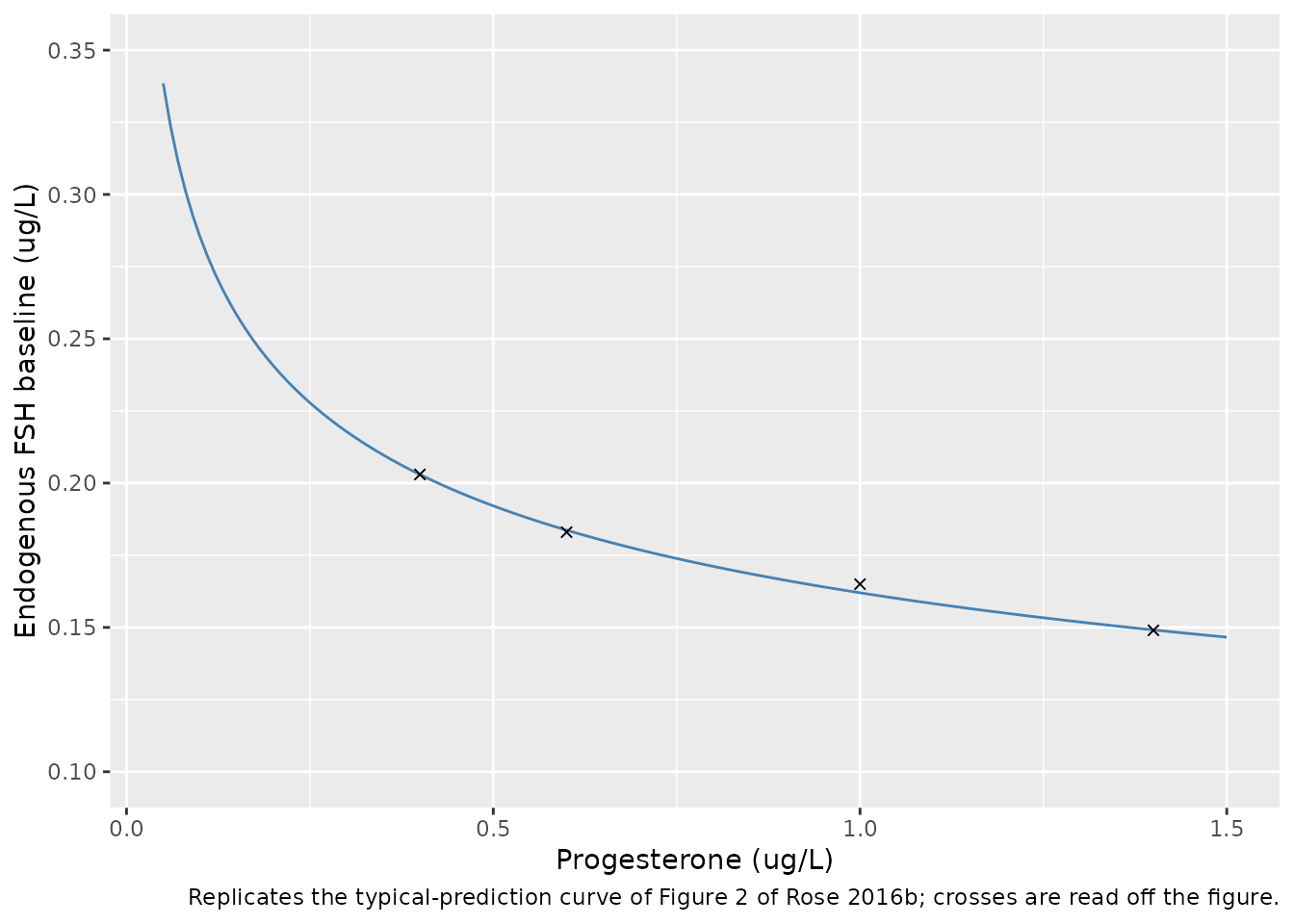
Figure 3: visual predictive check of total FSH
Replicates Figure 3. The paper’s VPC used 1000 replicates of the 24-subject trial; here one cohort of 200 virtual subjects is simulated. The residual error magnitudes are not published, so the simulated percentiles carry between-subject variability only and are expected to be narrower than the observed 2.5th-97.5th percentile band. The observed medians below were digitised from the Figure 3 median line by the maintainers against the printed axis ticks (about 0.01 ug/L resolution).
fig3_median <- tibble::tribble(
  ~day, ~median_obs,
  0,    0.198,
  1,    0.605,
  2,    0.790,
  3,    1.035,
  4,    1.087,
  5,    1.216,
  6,    1.210,
  6.5,  1.334,
  7,    1.275,
  8,    0.875,
  9,    0.605,
  10,   0.416,
  11,   0.292,
  12,   0.224,
  13,   0.176,
  14,   0.170,
  15,   0.176
)

vpc <- sim |>
  dplyr::mutate(day = time / 24) |>
  dplyr::group_by(day) |>
  dplyr::summarise(
    p025 = stats::quantile(Cc, 0.025),
    p50 = stats::median(Cc),
    p975 = stats::quantile(Cc, 0.975),
    .groups = "drop"
  )

ggplot(vpc, aes(day)) +
  geom_ribbon(aes(ymin = p025, ymax = p975), fill = "lightblue", alpha = 0.6) +
  geom_line(aes(y = p50), colour = "steelblue") +
  geom_line(data = typ, aes(time / 24, Cc), colour = "black", linetype = "dashed") +
  geom_point(data = fig3_median, aes(day, median_obs), shape = 4, size = 2) +
  labs(x = "Time after first dose (days)", y = "Total FSH concentration (ug/L)",
       caption = paste("Replicates Figure 3 of Rose 2016b. Ribbon: simulated 2.5th-97.5th",
                       "percentiles; solid: simulated median; dashed: typical value;",
                       "crosses: digitised observed median."))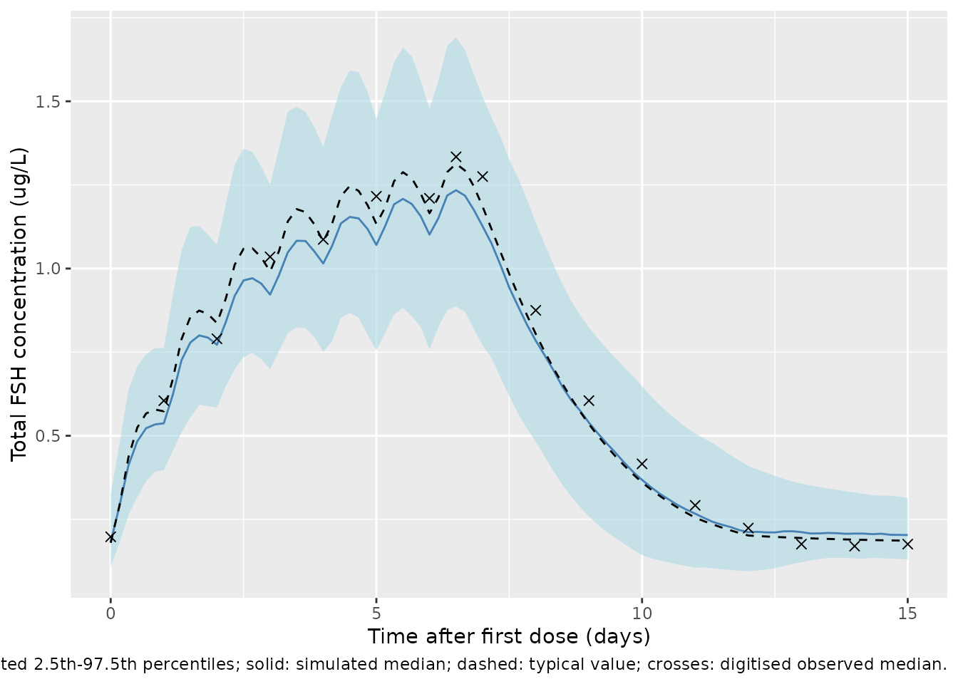
fig3_cmp <- fig3_median |>
  dplyr::left_join(vpc |> dplyr::select(day, p50), by = "day") |>
  dplyr::mutate(pct_diff = 100 * (p50 - median_obs) / median_obs)
knitr::kable(fig3_cmp |>
               dplyr::rename("Day" = day, "Observed median (Fig. 3)" = median_obs,
                             "Simulated median" = p50, "% diff" = pct_diff),
digits = 3)| Day | Observed median (Fig. 3) | Simulated median | % diff |
|---|---|---|---|
| 0.0 | 0.198 | 0.182 | -8.083 |
| 1.0 | 0.605 | 0.537 | -11.187 |
| 2.0 | 0.790 | 0.772 | -2.270 |
| 3.0 | 1.035 | 0.922 | -10.919 |
| 4.0 | 1.087 | 1.015 | -6.606 |
| 5.0 | 1.216 | 1.071 | -11.963 |
| 6.0 | 1.210 | 1.102 | -8.960 |
| 6.5 | 1.334 | 1.234 | -7.491 |
| 7.0 | 1.275 | 1.126 | -11.678 |
| 8.0 | 0.875 | 0.784 | -10.374 |
| 9.0 | 0.605 | 0.539 | -10.850 |
| 10.0 | 0.416 | 0.368 | -11.490 |
| 11.0 | 0.292 | 0.267 | -8.542 |
| 12.0 | 0.224 | 0.212 | -5.502 |
| 13.0 | 0.176 | 0.212 | 20.419 |
| 14.0 | 0.170 | 0.208 | 22.114 |
| 15.0 | 0.176 | 0.203 | 15.480 |
The simulated median reproduces the shape and timing of the observed median: the rise over the dosing week, the peak 12 h after the last dose, and the elimination-limited washout. It runs about 5-12 % below the observed median from day 1 to day 12 and about 15-22 % above it on days 13-15. Both offsets track the illustrative inhibin B input rather than the PK parameters. Endogenous FSH contributes up to 0.18 ug/L of the total, so how deeply and how long inhibin B suppresses it moves the total by roughly 0.1 ug/L; the scenario’s inhibin B returns to baseline by day 12, so endogenous FSH recovers faster than it did in the trial, where the observed day-15 median (0.176 ug/L) was still below the day-0 median (0.198 ug/L). The typical-value profile for a 65 kg woman reaches 1.313 ug/L at day 6.5 against the observed median peak of 1.334 ug/L.
The checks below use the centre of the comparison and a robust quantile rather than the worst single day, since the cohort’s tails are not reproducible across rxode2 builds. The bounds leave room for the inhibin B scenario offsets described above; a mis-transcribed clearance, volume, dose or unit shifts the whole profile by tens of percent and still fails them.
typ_peak <- typ |> dplyr::filter(time > 0) |> dplyr::slice_max(Cc, n = 1)
typ_peak
#>   time       Cc     rbase    Cc_endo   Cc_exo
#> 1  156 1.313152 0.1799741 0.04714061 1.266012
stopifnot(
  abs(median(fig3_cmp$pct_diff)) < 15,
  stats::quantile(abs(fig3_cmp$pct_diff), 0.9) < 35,
  # Figure 3 observed median peak, 1.334 ug/L at day 6.5.
  abs(typ_peak$Cc - 1.334) / 1.334 < 0.10,
  typ_peak$time >= 144, typ_peak$time <= 168
)
Figure 5: endogenous FSH suppressed by inhibin B
Replicates the mechanism of Figure 5: the model-predicted endogenous FSH (solid) falls well below the observed baseline (dashed) as inhibin B (purple, right axis) rises, and recovers when inhibin B returns to baseline. Six virtual subjects are shown.
show_ids <- sort(unique(sim$id))[1:6]
inhb_scale <- 0.4 / 6000
fig5 <- sim |>
  dplyr::filter(id %in% show_ids) |>
  dplyr::mutate(day = time / 24)
ggplot(fig5, aes(day)) +
  geom_line(aes(y = Cc_endo), colour = "steelblue") +
  geom_hline(data = fig5 |> dplyr::distinct(id, rbase),
             aes(yintercept = rbase), colour = "steelblue", linetype = "dashed") +
  geom_line(aes(y = INHIBINB * inhb_scale), colour = "purple") +
  scale_y_continuous("Endogenous FSH (ug/L)",
                     sec.axis = sec_axis(~ . / inhb_scale, name = "Inhibin B (pg/mL)")) +
  facet_wrap(~id) +
  labs(x = "Time after first dose (days)",
       caption = "Replicates the layout of Figure 5 of Rose 2016b with illustrative inhibin B profiles.")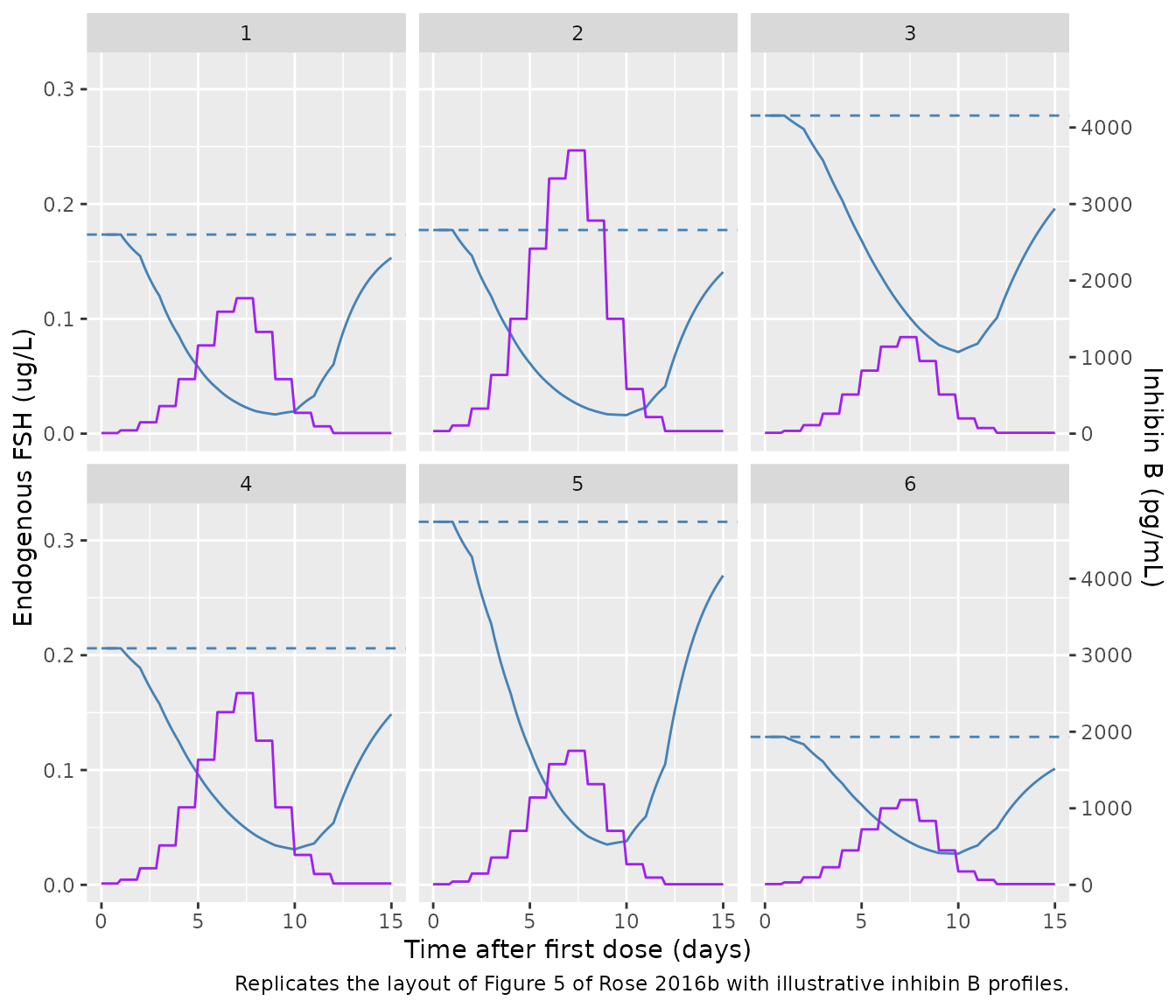
typ_nadir <- min(typ$Cc_endo)
c(baseline = typ$rbase[1], nadir = typ_nadir, day15 = typ$Cc_endo[nrow(typ)])
#>   baseline      nadir      day15
#> 0.17997414 0.02424716 0.14457027
stopifnot(
  # Deterministic typical-value solve: endogenous FSH never exceeds its
  # baseline after t = 0 because inhibin B never falls below its baseline.
  all(typ$Cc_endo[typ$time > 0] <= typ$rbase[1] * (1 + 1e-6)),
  typ_nadir < 0.25 * typ$rbase[1]
)
PKNCA: exogenous FE 999049 after the last dose
The paper reports no NCA table of its own; its only exposure summary is the 40 h terminal half-life implied by CL/F and V/F. PKNCA is therefore run on the exogenous FE 999049 component (total minus endogenous) over the last dosing interval (day 6, 144-168 h) and on the terminal phase from the last dose to day 15, and the half-life is compared with the paper’s value.
conc_df <- sim |>
  dplyr::filter(!is.na(Cc_exo)) |>
  dplyr::select(id, time, treatment, Cc_exo)
dose_df <- events_total |>
  dplyr::filter(evid == 1, time == 144) |>
  dplyr::select(id, time, treatment, amt)

conc_obj <- PKNCA::PKNCAconc(conc_df, Cc_exo ~ time | treatment + id,
                             concu = "ug/L", timeu = "h")
dose_obj <- PKNCA::PKNCAdose(dose_df, amt ~ time | treatment + id, doseu = "ug")
intervals <- data.frame(
  start = c(144, 144),
  end = c(168, 360),
  cmax = c(TRUE, FALSE),
  tmax = c(TRUE, FALSE),
  auclast = c(TRUE, FALSE),
  half.life = c(FALSE, TRUE)
)
nca_res <- PKNCA::pk.nca(PKNCA::PKNCAdata(conc_obj, dose_obj, intervals = intervals))
summary(nca_res)
#>  Interval Start Interval End                  treatment   N AUClast (h*ug/L)
#>             144          168 225 IU (13.1 ug) SC QD x 7 200      26.9 [17.1]
#>             144          360 225 IU (13.1 ug) SC QD x 7 200                .
#>  Cmax (ug/L)          Tmax (h) Half-life (h)
#>  1.17 [17.1] 12.0 [8.00, 20.0]             .
#>            .                 .   43.2 [10.5]
#>
#> Caption: AUClast, Cmax: geometric mean and geometric coefficient of variation; Tmax: median and range; Half-life: arithmetic mean and standard deviation; N: number of subjects

published <- tibble::tibble(treatment = "225 IU (13.1 ug) SC QD x 7", half.life = 40)
cmp <- nlmixr2lib::ncaComparisonTable(
  simulated = nca_res,
  reference = published,
  by = "treatment",
  units = c(half.life = "h"),
  tolerance_pct = 20
)
knitr::kable(cmp, caption = "Simulated vs. published terminal half-life. * differs from reference by >20%.")| NCA parameter | treatment | Reference | Simulated | % diff |
|---|---|---|---|---|
| t½ (h) | 225 IU (13.1 ug) SC QD x 7 | 40 | 42.2 | +5.6% |
The simulated terminal half-life of the exogenous component agrees
with the paper’s 40 h: the dosing-site and transit rate constants (0.329
and 0.148 1/h) are much faster than elimination (0.0174 1/h), so the
terminal phase is elimination-limited. The simulated median is slightly
longer, partly because the paper’s 40 h refers to a 65 kg woman while
the virtual cohort averages 71.5 kg and kel scales with
WT^-0.25 (about 2 %), and partly because PKNCA’s best-fit
terminal window can start while absorption is still contributing.
Assumptions and deviations
-
Residual error. The paper used a combined additive
and proportional residual error model but does not report either
magnitude. Both are encoded as
fixed(0); the companion single-dose model’s values (0.038 ug/L, 0.033) were not carried across because they come from a different fit. Simulated observation percentiles therefore reflect between-subject variability only. - CL/F - V/F covariance. Reported as positive and significant (Table 3, dOFV 11.77) but its magnitude is not printed; the IIV block is diagonal.
-
IIV scale. Table 2 reports IIV as CV% without
confidence intervals, so it cannot show whether the percentages are
exact log-normal CVs or
100 * omega. Variances were computed aslog(CV^2 + 1), matching the companion single-dose model. Under the100 * omegareading they would be(CV/100)^2; the two differ by under 4 % for CL/F, V/F and FSHbl but by 32 % for ktr (0.528 versus 0.696). - Progesterone reference. The power function is un-normalised (reference 1 ug/L), as identified by the Figure 2 curve passing through FSHbl at progesterone 1.0 ug/L.
-
kin back-calculation. The paper states that
kinis calculated from the pre-dose steady state of the other parameters and baseline values but prints no formula; setting Eq. 8 to zero at t = 0 with the central amount atFSHbl * V/Fgives the expression in the model, which requires the t = 0 inhibin B as the separate time-fixed columnINHIBINB_BASE. - Dose in mass units. The paper gives only 225 IU; 13.1 ug is the specific-activity conversion printed in the companion single-dose paper.
-
Inhibin B time course. Not tabulated in the paper.
The vignette uses an illustrative daily profile shaped after Figure 5,
carried forward between daily values as the paper did (Section 2.1); it
is a scenario input, not a fitted quantity. Solve with
covsInterpolation = "locf"to reproduce the paper’s handling of the daily inhibin B samples. - Covariate distributions. Table 1 gives means and ranges only; weight is drawn as normal and progesterone, baseline inhibin B and the inhibin B peak as log-normal, truncated to the published ranges.
-
Covariate names. Baseline progesterone
(
PROG_BASE), time-varying inhibin B (INHIBINB) and baseline inhibin B (INHIBINB_BASE) were added to the covariate register for this model, following the time-fixed<X>_BASEpattern ofCRCL_BASE.