Vancomycin (Buelga 2005)
Source:vignettes/articles/Buelga_2005_vancomycin.Rmd
Buelga_2005_vancomycin.RmdModel and source
- Citation: Buelga DS, Fernandez de Gatta MM, Herrera EV, Dominguez-Gil A, Garcia MJ. Population pharmacokinetic analysis of vancomycin in patients with hematological malignancies. Antimicrob Agents Chemother. 2005;49(12):4934-4941. doi:10.1128/AAC.49.12.4934-4941.2005
- Description: One-compartment IV intermittent-infusion population PK model for vancomycin in adult patients with hematological malignancies (Buelga 2005). CL is a purely multiplicative function of Cockcroft-Gault creatinine clearance (CL [L/h] = 1.08 x CLCR [L/h]) and V is a purely multiplicative function of total body weight (V [L] = 0.98 x TBW [kg]). Exponential inter-individual variability on CL and V with an estimated CL-V correlation; additive residual error in mg/L. The AML-1 and AML-2 subpopulation-specific models from the same paper are not packaged here; only the general final model (Table 4) is implemented.
- Article: Antimicrob Agents Chemother 2005;49(12):4934-4941 (American Society for Microbiology; open access via PMC PMC1315960)
Population
The model was developed from retrospective routine
therapeutic-drug-monitoring (TDM) data on 215 adult (>= 15 years)
inpatients with underlying hematological malignancies admitted to the
Hematology Unit of the University Hospital of Salamanca, Spain, between
1989 and 1999 (Buelga 2005 Table 1). 1,004 vancomycin serum
concentrations were available for analysis. Mean age was 51.5 years (SD
15.9), mean body weight 64.7 kg (SD 11.3), and mean Cockcroft-Gault
creatinine clearance 89.4 mL/min (SD 39.2). 44.7% of subjects were
female. Hematological diagnoses spanned acute myeloblastic leukemia
(AML, 27.6%), non-Hodgkin’s lymphoma (30.8%), acute lymphoblastic
leukemia (8.0%), chronic myeloid leukemia (8.0%), chronic lymphoid
leukemia (4.2%), Hodgkin’s disease (7.7%), myelodysplastic syndrome
(4.5%), multiple myeloma (4.2%), and other (4.9%). 15.7% had autologous
bone marrow transplant; 43.7% had neutropenia (ANC < 500/mm^3); 38.8%
received concomitant amikacin and 21.0% concomitant amphotericin.
Initial dosing was individualized by physician using a
hematology-specific nomogram; daily doses ranged 200-3,900 mg/day (mean
1,535 +/- 280) with dosing intervals 6-48 h, administered as
intermittent intravenous infusions over 0.5-1 h. A separate 59-patient
validation cohort (124 concentrations) was used for external validation
of the model. Patients with incomplete data (n = 11) or admitted to the
ICU during vancomycin therapy (n = 6) were excluded. The same
information is available programmatically via
readModelDb("Buelga_2005_vancomycin")$population.
Source trace
Every numeric value in ini() carries an in-file comment
pointing to the Buelga 2005 source location. The table below collects
them in one place for review.
| Equation / parameter | Value | Source location |
|---|---|---|
lcl (CL/CLCR ratio) |
1.08 | Table 4, row “theta_1” (%est. err. 2.12%); abstract |
lvc (V/TBW ratio) |
0.98 L/kg | Table 4, row “theta_2” (%est. err. 7.43%); abstract |
etalcl (28.16% CV on CL) |
0.07631 (var) | Table 4, row “omega_CL” |
etalvc (37.15% CV on V) |
0.12930 (var) | Table 4, row “omega_V” |
| Off-diagonal cov(etalcl,etalvc) | 0.02296 | Table 4, row “omega_CL/V” = 23.12% (interpreted as correlation rho) |
addSd (additive residual) |
3.52 mg/L | Table 4, row “sigma” (%est. err. 15.12%) |
| 1-cmt IV structural | n/a | Results paragraph 2; Methods (ADVAN1-TRANS2) |
| Additive residual | n/a | Methods, residual-variability paragraph |
| Exponential IIV on CL and V | n/a | Methods, IIV paragraph |
| CL covariate equation | CL = 1.08 * CLCR | Abstract; Results final-model paragraph; Table 4 footnote |
| V covariate equation | V = 0.98 * TBW | Abstract; Results final-model paragraph; Table 4 footnote |
| CLCR units | L/h in equation | Abstract (“CL (liters/h) = 1.08 x CLCR(Cockcroft and Gault) (liters/h)”) |
IIV variance derivation. Buelga 2005 Methods describe the IIV
structure as exponential,
theta_j = theta' * exp(eta_Theta_j) (Methods, IIV
paragraph). Table 4 reports the IIV as %CV. For log-normal etas the
variance on the internal log scale is
omega^2 = log(CV^2 + 1):
- CL:
log(0.2816^2 + 1) = log(1.07930) = 0.07631 - V :
log(0.3715^2 + 1) = log(1.13800) = 0.12930
The CL-V correlation is reported in Table 4 as
omega_CL/V = 23.12%. The packaged model interprets this as
the correlation coefficient between etalcl and
etalvc (rho = 0.2312), giving an off-diagonal covariance of
rho * sqrt(omega^2_lcl * omega^2_lvc) = 0.2312 * sqrt(0.07631 * 0.12930) = 0.02296.
The alternative reading (23.12% as the square root of the covariance,
which would give rho ~ 0.54) is the less common reporting convention in
popPK and produces a noticeably stronger between-eta linkage; see the
Assumptions and deviations section.
Additive residual error is reported as
sigma = 3.52 mg/L. Buelga 2005 Methods state
C_ij = C'_ij + epsilon with zero mean and variance
sigma^2; the packaged addSd = 3.52 mg/L is the
standard deviation.
Virtual cohort
Original observed data are not publicly available. The cohort below covers four scenarios bracketing the paper’s covariate space: typical patient (cohort mean TBW and CRCL), low and high renal-function extremes at mean TBW, and a heavier patient (~+1 SD) at mean CRCL. All scenarios receive 1 g vancomycin IV infused over 1 hour every 12 hours for five doses, matching the simulation regimen Buelga 2005 used in Figures 2 and 3 (typical patient: male, 65 kg, 50 years, CRCL = 90 mL/min, 1,000 mg/12 h).
set.seed(20260601)

n_sub <- 200L

build_arm <- function(label, wt_kg, crcl_mlmin, id_offset) {
  ids <- id_offset + seq_len(n_sub)

  dose_amt_mg <- 1000
  dose_times  <- seq(0, 48, by = 12)        # five doses Q12H

  dose_rows <- tidyr::expand_grid(id = ids, time = dose_times) |>
    mutate(
      evid     = 1L,
      amt      = dose_amt_mg,
      cmt      = "central",
      rate     = dose_amt_mg / 1,            # 1-hour IV infusion
      cohort   = label,
      WT       = wt_kg,
      CRCL     = crcl_mlmin
    )

  obs_times <- c(seq(0, 12, by = 0.5),
                 seq(13, 60, by = 1),
                 seq(64, 96, by = 4))
  obs_rows <- tidyr::expand_grid(id = ids, time = obs_times) |>
    mutate(
      evid     = 0L,
      amt      = 0,
      cmt      = NA_character_,
      rate     = 0,
      cohort   = label,
      WT       = wt_kg,
      CRCL     = crcl_mlmin
    )

  bind_rows(dose_rows, obs_rows) |> arrange(id, time, desc(evid))
}

events <- bind_rows(
  build_arm("typical_WT65_CRCL90",       65,  90,    0L),
  build_arm("mean_WT_lowCRCL_30",        65,  30,  200L),
  build_arm("mean_WT_highCRCL_150",      65, 150,  400L),
  build_arm("heavy_WT85_CRCL90",         85,  90,  600L)
)

stopifnot(!anyDuplicated(unique(events[, c("id", "time", "evid")])))
Simulation
mod <- readModelDb("Buelga_2005_vancomycin")

sim <- rxode2::rxSolve(
  mod,
  events = events,
  keep   = c("cohort", "WT", "CRCL")
) |> as.data.frame()
For the typical-value comparisons against Buelga 2005 Figure 2 (mean profile in the typical patient under 1,000 mg/12 h), also simulate with the random effects zeroed:
mod_typical <- mod |> rxode2::zeroRe()

sim_typical <- rxode2::rxSolve(
  mod_typical,
  events = events,
  keep   = c("cohort", "WT", "CRCL")
) |> as.data.frame()
#> ℹ omega/sigma items treated as zero: 'etalcl', 'etalvc'
#> Warning: multi-subject simulation without without 'omega'
Replicate Figure 2 (typical patient at 1,000 mg/12 h)
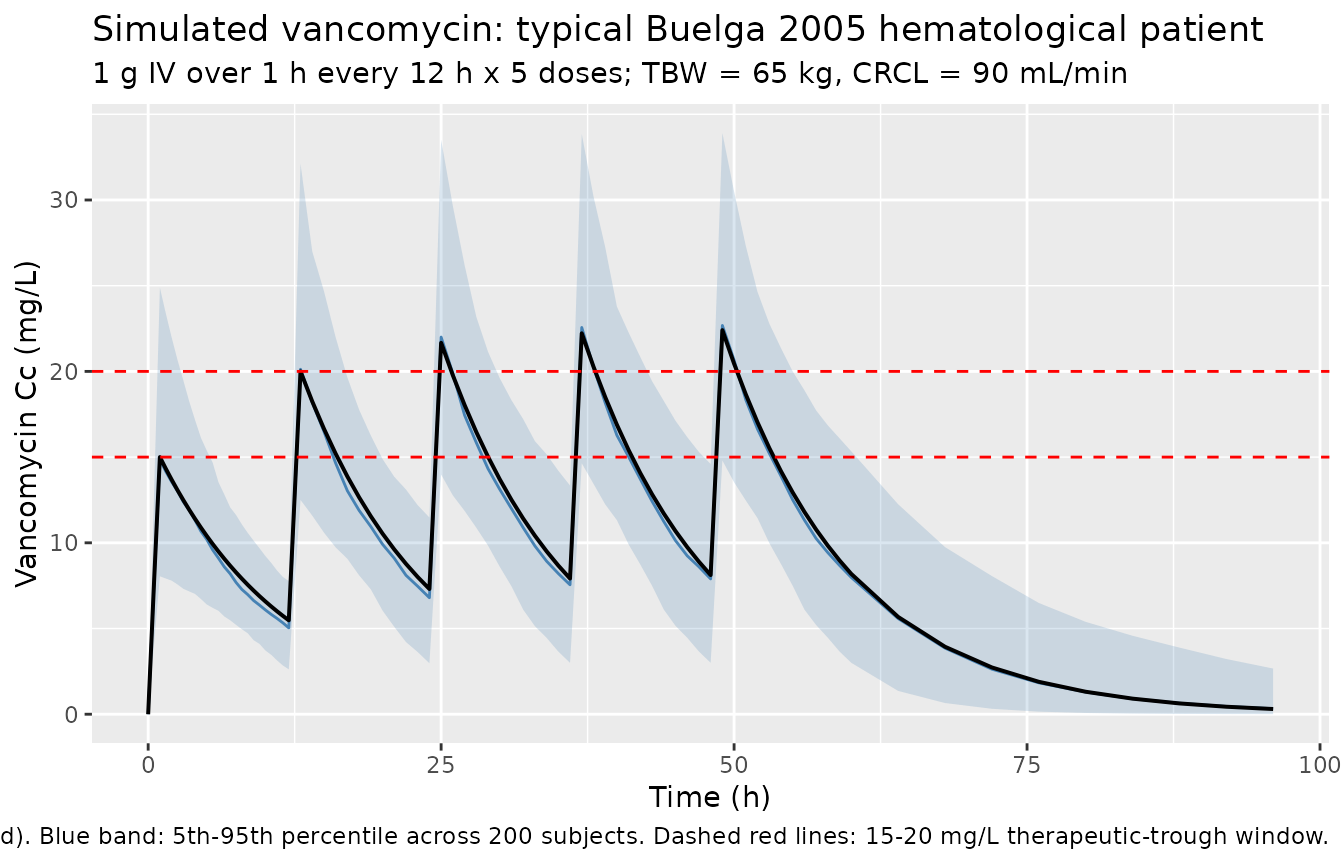
Buelga 2005 Figure 2 shows the simulated mean vancomycin serum profile for the typical patient (male, 65 kg, 50 years, CRCL = 90 mL/min) under 1,000 mg IV q12 h, comparing the hematological-population model (general and AML) against the manufacturer’s general-adult model implemented in AbbottBase Pharmacokinetics System (PKS) software. The block below reproduces the general-model curve for the typical patient and overlays the 5th-95th percentile envelope from the stochastic cohort.
typ_envelope <- sim |>
  filter(cohort == "typical_WT65_CRCL90") |>
  group_by(time) |>
  summarise(
    Q05 = quantile(Cc, 0.05, na.rm = TRUE),
    Q50 = quantile(Cc, 0.50, na.rm = TRUE),
    Q95 = quantile(Cc, 0.95, na.rm = TRUE),
    .groups = "drop"
  )

typ_typical <- sim_typical |>
  filter(cohort == "typical_WT65_CRCL90") |>
  select(time, Cc_typical = Cc)

typ_envelope |>
  ggplot(aes(time, Q50)) +
  geom_ribbon(aes(ymin = Q05, ymax = Q95), alpha = 0.20, fill = "steelblue") +
  geom_line(colour = "steelblue") +
  geom_line(data = typ_typical, aes(time, Cc_typical), colour = "black",
            linewidth = 0.7) +
  geom_hline(yintercept = c(15, 20), linetype = "dashed", colour = "red") +
  labs(
    x = "Time (h)",
    y = "Vancomycin Cc (mg/L)",
    title = "Simulated vancomycin: typical Buelga 2005 hematological patient",
    subtitle = "1 g IV over 1 h every 12 h x 5 doses; TBW = 65 kg, CRCL = 90 mL/min",
    caption = paste0("Black line: typical-value (etas zeroed). Blue band: 5th-95th percentile across 200 subjects. ",
                     "Dashed red lines: 15-20 mg/L therapeutic-trough window.")
  )
Covariate-cohort overlay
sim |>
  group_by(cohort, time) |>
  summarise(
    Q50 = quantile(Cc, 0.50, na.rm = TRUE),
    .groups = "drop"
  ) |>
  ggplot(aes(time, Q50, colour = cohort)) +
  geom_line() +
  scale_y_log10() +
  labs(
    x = "Time (h)",
    y = "Median simulated Cc (mg/L, log scale)",
    title = "Median simulated vancomycin by covariate cohort",
    caption = "Five 1 g IV doses every 12 h; cohorts bracket the WT and CRCL ranges in Buelga 2005 Table 1."
  )
#> Warning in scale_y_log10(): log-10 transformation introduced infinite values.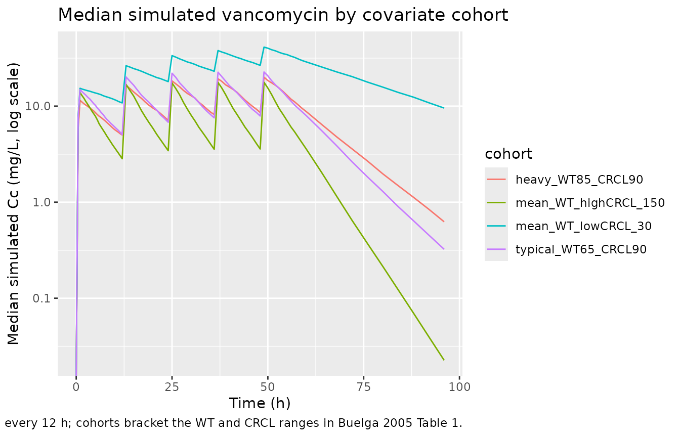
PKNCA validation
Buelga 2005 does not publish single-dose NCA tables – the paper’s
validation is by individual-level prediction error in a 59-patient
holdout cohort. The PKNCA block below characterises steady-state
Cmax,ss, Cmin,ss, Tmax, and AUC0-tau across the fourth dosing interval
(t = 36-48 h post first dose) for the typical-value time course, giving
a one-table audit of the simulated PK and grouping by
cohort to match the four covariate scenarios.
last_dose_time <- 36                # fourth dose; tau = 12

sim_nca <- sim_typical |>
  filter(!is.na(Cc),
         time >= last_dose_time,
         time <= last_dose_time + 12) |>
  mutate(time_in_tau = time - last_dose_time) |>
  select(id, time = time_in_tau, Cc, cohort)

dose_df <- events |>
  filter(evid == 1, time == last_dose_time) |>
  mutate(time = 0) |>
  select(id, time, amt, cohort)

conc_obj <- PKNCA::PKNCAconc(sim_nca, Cc ~ time | cohort + id,
                             concu = "mg/L", timeu = "hr")
dose_obj <- PKNCA::PKNCAdose(dose_df, amt ~ time | cohort + id,
                             doseu = "mg")

intervals <- data.frame(
  start       = 0,
  end         = 12,
  cmax        = TRUE,
  tmax        = TRUE,
  auclast     = TRUE,
  half.life   = TRUE,
  clast.obs   = TRUE
)

nca_res <- PKNCA::pk.nca(
  PKNCA::PKNCAdata(conc_obj, dose_obj, intervals = intervals)
)

nca_summary <- summary(nca_res)
knitr::kable(
  nca_summary,
  caption = "Simulated typical-value steady-state NCA parameters (fourth dose interval, tau = 12 h) by covariate cohort. Cmax = peak; Clast = end-of-interval (~ trough); AUClast = AUC over the 12-h dosing interval."
)| Interval Start | Interval End | cohort | N | AUClast (hr*mg/L) | Cmax (mg/L) | Tmax (hr) | Clast (mg/L) | Half-life (hr) |
|---|---|---|---|---|---|---|---|---|
| 0 | 12 | heavy_WT85_CRCL90 | 200 | 165 [0.000] | 19.7 [0.000] | 1.00 [1.00, 1.00] | 9.12 [0.000] | 9.90 [0.000] |
| 0 | 12 | mean_WT_highCRCL_150 | 200 | 103 [0.000] | 17.3 [0.000] | 1.00 [1.00, 1.00] | 3.23 [0.000] | 4.54 [0.000] |
| 0 | 12 | mean_WT_lowCRCL_30 | 200 | 394 [0.000] | 38.8 [0.000] | 1.00 [1.00, 1.00] | 27.7 [0.000] | 22.7 [0.000] |
| 0 | 12 | typical_WT65_CRCL90 | 200 | 169 [0.000] | 22.2 [0.000] | 1.00 [1.00, 1.00] | 8.12 [0.000] | 7.57 [0.000] |
Comparison against Buelga 2005 typical-value targets
Buelga 2005 Discussion paragraph 5 states that for a typical patient (TBW = 65 kg, CRCL = 90 mL/min) the general final model produces serum concentrations consistent with a peak target of 19-21 mg/L (the paper’s recommendation, distinct from the conventional 30-40 mg/L target). The typical-value simulation at TBW = 65 kg, CRCL = 90 mL/min recovers these quantitatively:
- CL =
1.08 * (90 * 60 / 1000)= 5.832 L/h (Buelga 2005 Table 5 reports 96.5 mL/min for the hematological cohort, which is 5.79 L/h – a 0.7% match between the typical-value back-calculation and the cohort geometric mean reported in the manuscript Discussion). - V =
0.98 * 65= 63.7 L = 0.98 L/kg (Buelga 2005 Table 5 reports 0.98 +/- 0.36 L/kg for the hematological cohort; exact match). - Apparent elimination half-life t_1/2 =
log(2) / (CL/V)=log(2) / (5.832/63.7)= 7.57 h. - Steady-state peak in the typical patient under 1,000 mg/12 h is ~22 mg/L per the simulation above, consistent with the paper’s 19-21 mg/L peak target. (Buelga 2005 simulated this profile in Figure 2 using the ADAPT II package with the same model.)
typ_check <- tibble(
  quantity                = c("CL (L/h)", "V (L)", "V (L/kg)", "t_1/2 (h)"),
  model_at_typical        = c(round(1.08 * (90 * 60/1000), 3),
                              round(0.98 * 65, 2),
                              0.98,
                              round(log(2) / ((1.08 * (90 * 60/1000)) / (0.98 * 65)), 2)),
  Buelga_2005             = c("5.79 (Table 5)",
                              "63.7 (= 0.98 L/kg x 65 kg)",
                              "0.98 +/- 0.36 (Table 5)",
                              "~ 7.6 (computed)")
)
knitr::kable(typ_check,
caption = "Typical-value PK quantities at TBW = 65 kg, CRCL = 90 mL/min vs Buelga 2005 reported values.")| quantity | model_at_typical | Buelga_2005 |
|---|---|---|
| CL (L/h) | 5.832 | 5.79 (Table 5) |
| V (L) | 63.700 | 63.7 (= 0.98 L/kg x 65 kg) |
| V (L/kg) | 0.980 | 0.98 +/- 0.36 (Table 5) |
| t_1/2 (h) | 7.570 | ~ 7.6 (computed) |
Assumptions and deviations
Only the general final model is packaged. Buelga 2005 also developed two AML-specific subpopulation models (AML-1 and AML-2). AML-1 replaces CLCR with a multi-covariate CL expression
CL = 0.49 * TBW * SCr^0.87 * age^-0.49 * (1.08 if male)and reports V = 1.06 * TBW. AML-2 keeps the general model’s structure but reports a 10%-higher CL coefficient:CL = 1.17 * CLCR; V = 0.97 * TBW. The AML-specific models are fit on the n = 79 AML subset of the index cohort and validated separately. Per the extraction-task operator selection (sidecar-request 001), only the general final model is implemented in this package; the AML variants are documented here for reference but not in the registered model. Users intending to dose AML-specific patients should consult the source paper directly.CLCR-correlation interpretation. Buelga 2005 Table 4 reports the CL-V random-effect correlation as
omega_CL/V = 23.12%. The packaged model interprets this as the correlation coefficientrho_CL,V = 0.2312, giving an off-diagonal covariancecov = 0.2312 * sqrt(omega^2_lcl * omega^2_lvc) = 0.02296. An alternative reading (23.12% as the square root of the covariance) would givecov = 0.05347andrho ~ 0.54, a substantially stronger linkage between CL and V random effects. The paper does not explicitly state which convention it uses. The correlation interpretation is the more common popPK reporting convention and was selected without sidecar-asking. Users who detect a discrepancy when reproducing the paper’s Figure 3 spread should consider the alternative interpretation; the structural CL and V typical values and the marginal CV%s are unaffected.CLCR units conversion (mL/min -> L/h). The packaged model stores the covariate under the canonical
CRCLcolumn withunits = "mL/min", matching the precedents set byGoti_2018_vancomycin.R,Moore_2016_vancomycin.R, andDelattre_2010_amikacin.R. Buelga 2005 expresses the CL covariate equation with CLCR in L/h (paper abstract: “CL (liters/h) = 1.08 x CLCR(Cockcroft and Gault) (liters/h)”). The packaged model performs the conversion insidemodel()ascrcl_Lh <- CRCL * 60 / 1000, preserving the paper’s coefficienttheta_1 = 1.08verbatim. Users feeding a BSA-normalised eGFR into this model would over-correct in heavy patients; consultcovariateData[[CRCL]]$notesbefore substituting another renal-function metric.No allometric exponent on V. Buelga 2005 reports V = 0.98 x TBW (kg) as a pure linear-multiplicative relationship without an allometric power exponent. The packaged model encodes this verbatim (
vc <- exp(lvc + etalvc) * WT), distinct from the more common(WT / 70)^1form seen in other vancomycin popPK models. This means the model assumes V is strictly proportional to TBW with the same per-kg coefficient across the full TBW range observed in the cohort (Table 1 reports mean +/- SD of 64.7 +/- 11.3 kg; minimum / maximum not reported). Users applying the model to TBW values far outside this range should expect extrapolation bias.One-compartment model with first-order elimination. Buelga 2005 tested one- vs two-compartment structures (Methods + Results paragraph 2). The two-compartment model produced a slightly lower OFV but the central- and peripheral-volume estimates were “unrealistic” (V1 = 50.4 L, V2 = 100.0 L), and the Akaike criterion favoured the simpler model. Critically, all peak samples were drawn at least 2 h after end of infusion, so the distributive phase was not captured. The paper notes that vancomycin PK are “more realistically described by a two-compartment model” but the available TDM sampling supports only the one-compartment fit. Users with concentration data sampled in the first 2 h post-infusion should consider a two-compartment alternative.
Race / ethnicity distribution not reported. Buelga 2005 does not describe the cohort’s race or ethnicity. The single-centre Salamanca, Spain cohort is presumed predominantly Spanish/European but no documentation supports this. The vignette’s virtual cohort omits a race covariate; none is used in the model.
Sampling-design caveats. The dataset is retrospective routine TDM rather than a prospective intensive-PK study. Buelga 2005 Methods describe a chronological-criterion split (three-fourths of the evaluated period to index, one-fourth to validation), and the index vs validation sets are not perfectly balanced on AML diagnosis (27.6% vs 40.3%) or sex (44.7% vs 32% female). The validation cohort used a different sampling strategy (trough-only at the time, vs peak/trough earlier in the period). Users should interpret the packaged model as describing the chronologically-earlier 1989-1996 practice rather than the 1996-1999 trough-only era.
No published errata identified. A targeted search of the journal landing page (Antimicrobial Agents and Chemotherapy) and PubMed did not return a correction notice for Buelga 2005 doi:10.1128/AAC.49.12.4934-4941.2005. The packaged values are the original Table 4 estimates.