Indium-based quantum dots (Yaghini 2021)
Source:vignettes/articles/Yaghini_2021_quantumDot.Rmd
Yaghini_2021_quantumDot.RmdModel and source
Yaghini et al. (2021) fitted two separate NONMEM models to indium concentrations measured by ICP-MS after a single intravenous dose of PEGylated, cadmium-free indium-phosphide quantum dots (bio CFQD) in female Balb/c mice:
-
Model A
(
Yaghini_2021_quantumDot_blood_mouse, Table 1, Figure 5): a two-compartment model of serum indium over the first 24 h. -
Model B
(
Yaghini_2021_quantumDot_organ_mouse, Table 2, Figures 1B and 8): a three-compartment model with blood, liver and spleen compartments over 90 days.
The authors describe the two as a two-step approach (“a distinct, separate model was required to describe tissue disposition”), so they are packaged as two model files.
- Citation: Yaghini E, Tacconi E, Pilling A, Rahman P, Broughton J, Naasani I, Keshtgar MRS, MacRobert A, Della Pasqua O. (2021). Population pharmacokinetic modelling of indium-based quantum dot nanoparticles: preclinical in vivo studies. Eur J Pharm Sci 157:105639. doi:10.1016/j.ejps.2020.105639.
- Description (Model A): Preclinical (mouse, female Balb/c). Two-compartment population PK model with first-order elimination for indium-based, cadmium-free PEGylated quantum dots (bio CFQD, InP core) after a single IV bolus, fitted to serum indium concentrations over the first 24 h. No between-animal variability (destructive and sparse sampling). The printed parameters do not reproduce the paper’s own Figure 5 profile; see the vignette Errata. Companion organ-disposition model: modellib(‘Yaghini_2021_quantumDot_organ_mouse’).
- Description (Model B): Preclinical (mouse, female Balb/c). Three-compartment population PK model of blood, liver and spleen disposition of indium-based, cadmium-free PEGylated quantum dots (bio CFQD, InP core) after a single IV bolus, fitted to indium concentrations over 90 days. Blood is the central compartment with first-order elimination; liver and spleen exchange with blood through intercompartmental clearances. No between-animal variability (destructive sampling). The printed parameters do not reproduce the paper’s own Figure 8 blood profile and the residual-error magnitudes are not reported; see the vignette Errata. Companion 0-24 h blood model: modellib(‘Yaghini_2021_quantumDot_blood_mouse’).
- Article: https://doi.org/10.1016/j.ejps.2020.105639 (open access, PMC8214104)
Read the Errata before using either model. The printed parameter tables are internally consistent in places (Table 2’s rate constants and blood and liver half-lives follow exactly from its flows and volumes), but neither table reproduces the paper’s own concentration-time figures. Both models are packaged as printed.
Population
Female Balb/c mice received 20 mg/kg quantum dots (200 uL in PBS) via the tail vein. Nine groups of three mice were sacrificed at 5 min, 1 h, 4 h and 1, 3, 10, 30, 60 and 90 days for blood and organ collection, and a separate set of three mice was sampled for serum at 5, 20, 40, 60 and 120 min (Methods 2.3). Indium was measured by ICP-MS in serum and in nitric-acid digests of 0.1 g tissue (Methods 2.5). No body weights and no analysis-dataset summary are reported. Figure 5 shows 21 serum observations at 7 times (the serial set plus the 4 h and 24 h groups, inferred 9 mice) for Model A; Figure 8 shows blood, liver and spleen from the nine groups plus the serial set (inferred 30 mice) for Model B. With destructive sampling and n = 3 per time, no between-animal variability was estimated in either model. A rat toxicology arm (12 and 48 mg/kg) had no PK sampling.
str(readModelDb("Yaghini_2021_quantumDot_organ_mouse")()$population)
#> List of 7
#>  $ species       : chr "mouse (female Balb/c)"
#>  $ n_subjects    : int 30
#>  $ n_studies     : int 1
#>  $ sex_female_pct: num 100
#>  $ disease_state : chr "healthy"
#>  $ dose_range    : chr "single IV bolus of 20 mg/kg PEGylated bio CFQD quantum dots (200 uL in PBS via the tail vein)"
#>  $ notes         : chr "The analysis dataset is not tabulated. Nine biodistribution groups of 3 mice were sacrificed at 5 min, 1 h, 4 h"| __truncated__
Source trace
| Equation / parameter | Value | Source location |
|---|---|---|
| Model A structure | 2-cmt, first-order elimination, IV bolus | Results 3.3 and Figure 1A |
Model A lcl
|
log(0.0416 L/h) | Table 1, CL |
Model A lvc
|
log(0.0027 L) | Table 1, V1 |
Model A lq
|
log(0.498 L/h) | Table 1, Q |
Model A lvp
|
log(0.068 L) | Table 1, V2 |
Model A propSd
|
sqrt(0.0686) = 0.262 | Table 1, ‘Proportional error 0.0686’; read as a variance per Methods eq (2) |
Model A addSd
|
sqrt(0.05) ng/L = 0.000224 ug/L | Table 1, ‘Additive error (ng/L) 0.05 (38%)’; read as a variance |
Model B d/dt(central)
|
k21*liver + k31*spleen - (k12 + k13 + kel)*central |
Eq (3) |
Model B d/dt(liver)
|
k12*central - k21*liver |
Eq (4) |
Model B d/dt(spleen)
|
k13*central - k31*spleen |
Eq (5) |
Model B k12, k21, k13,
k31, kel
|
q/vc, q/vp, q2/vc,
q2/vp2, cl/vc
|
Eqs (6)-(10) |
Model B lcl
|
log(0.0021 L/h) | Table 2, CL |
Model B lvc
|
log(3.41 L) | Table 2, Vb |
Model B lq
|
log(0.0018 L/h) | Table 2, QT1 (liver) |
Model B lvp
|
log(0.13 L) | Table 2, VT1 (liver) |
Model B lq2
|
log(0.1606 L/h) | Table 2, QT2 (spleen) |
Model B lvp2
|
log(0.22 L) | Table 2, VT2 (spleen) |
| Model B residual errors | fixed(0) |
Results: ‘proportional and additive error model’; values not printed |
QCO (1.07 L/h) and Vtot (3.65 L) are printed in Table 2 but enter the
model only through eqs (11)-(12) and the Figure 1B caption,
QT = Fd * QCO and VT = FV * (Vtot - Vb). The
flows and volumes they produce are themselves printed, so the packaged
model uses QT1, VT1, QT2 and VT2 directly.
Internal consistency of Table 2
Table 2 prints the rate constants and half-lives that follow from its flows and volumes. The packaged parameters reproduce all of them except the spleen half-life, which matches in hours rather than the printed days.
ui_b <- rxode2::rxode(readModelDb("Yaghini_2021_quantumDot_organ_mouse"))
th <- exp(ui_b$theta[c("lcl", "lvc", "lq", "lvp", "lq2", "lvp2")])
k <- c(
  K12 = th[["lq"]] / th[["lvc"]],
  K21 = th[["lq"]] / th[["lvp"]],
  K13 = th[["lq2"]] / th[["lvc"]],
  K31 = th[["lq2"]] / th[["lvp2"]],
  ke = th[["lcl"]] / th[["lvc"]]
)
table2_k <- c(K12 = 0.0005, K21 = 0.014, K13 = 0.047, K31 = 0.73, ke = 0.0006)

thalf <- tibble::tibble(
  quantity = c("Blood t1/2 (day)", "Liver t1/2 (day)", "Spleen t1/2 (day)", "Spleen t1/2 (h)"),
  derived = c(
    log(2) / k[["ke"]] / 24,
    log(2) / k[["K21"]] / 24,
    log(2) / k[["K31"]] / 24,
    log(2) / k[["K31"]]
  ),
  printed = c(47.0, 2.0, 1.0, 1.0)
)

tibble::tibble(
  quantity = paste(names(k), "(1/h)"),
  derived = k,
  printed = table2_k
) |>
  dplyr::bind_rows(thalf) |>
  dplyr::mutate(
    derived = vapply(derived, format, character(1), digits = 3),
    printed = vapply(printed, format, character(1), scientific = FALSE)
  ) |>
  dplyr::rename(
    "Quantity" = quantity,
    "From Table 2 flows and volumes" = derived,
    "Printed in Table 2" = printed
  ) |>
knitr::kable(caption = "Table 2 rate constants and half-lives. The spleen row printed as days matches only in hours.")| Quantity | From Table 2 flows and volumes | Printed in Table 2 |
|---|---|---|
| K12 (1/h) | 0.000528 | 0.0005 |
| K21 (1/h) | 0.0138 | 0.014 |
| K13 (1/h) | 0.0471 | 0.047 |
| K31 (1/h) | 0.73 | 0.73 |
| ke (1/h) | 0.000616 | 0.0006 |
| Blood t1/2 (day) | 46.9 | 47 |
| Liver t1/2 (day) | 2.09 | 2 |
| Spleen t1/2 (day) | 0.0396 | 1 |
| Spleen t1/2 (h) | 0.95 | 1 |
# The printed rate constants are the derived ones rounded to the precision shown.
stopifnot(
  all(abs(k / table2_k - 1) < 0.07),
  abs(thalf$derived[1] / 47.0 - 1) < 0.01,
  abs(thalf$derived[2] / 2.0 - 1) < 0.05,
  # Spleen: 0.95 h matches the printed '1.0' only as hours.
  abs(thalf$derived[4] / 1.0 - 1) < 0.06,
  thalf$derived[3] < 0.1
)
Simulation
The paper reports the dose as 20 mg/kg of quantum dot. The analyte is indium, whose mass fraction in the particle is not reported, and no body weights are given. The simulations below use a nominal 400 ug dose (20 mg/kg x 20 g) into the central compartment; both models are linear, so every concentration scales with this choice.
dose_ug <- 400

mod_a <- readModelDb("Yaghini_2021_quantumDot_blood_mouse")
mod_b <- readModelDb("Yaghini_2021_quantumDot_organ_mouse")

times_a <- sort(unique(c(0, seq(0.001, 0.1, by = 0.001), seq(0.1, 2, by = 0.01), seq(2, 24, by = 0.25))))
ev_a <- rxode2::et(amt = dose_ug, cmt = "central") |>
  rxode2::et(times_a, cmt = "central")
sim_a <- rxode2::rxSolve(mod_a, events = ev_a) |>
  as.data.frame() |>
  dplyr::mutate(id = 1L, model = "A")

times_b <- sort(unique(c(0, seq(1 / 60, 2, by = 1 / 60), seq(2, 48, by = 0.5), seq(48, 90 * 24, by = 6))))
# Multi-endpoint model (Cc, Cliver, Cspleen): observation rows carry dvid = 1
# and no cmt; every row returns all three outputs.
ev_b <- dplyr::bind_rows(
  data.frame(id = 1L, time = 0, amt = dose_ug, evid = 1L, cmt = "central", dvid = NA_integer_),
  data.frame(id = 1L, time = times_b, amt = 0, evid = 0L, cmt = NA_character_, dvid = 1L)
)
sim_b <- rxode2::rxSolve(mod_b, events = ev_b, rtol = 1e-10, atol = 1e-12) |>
  as.data.frame() |>
  dplyr::mutate(id = 1L, model = "B")
Mass balance (Model B)
Only kel removes indium from the system, so the amount
remaining in the three compartments plus the amount eliminated
(CL times the blood AUC) must equal the dose at every
time.
mb <- sim_b |>
  dplyr::arrange(time) |>
  dplyr::mutate(
    auc = c(0, cumsum(diff(time) * (head(Cc, -1) + tail(Cc, -1)) / 2)),
    eliminated = th[["lcl"]] * auc,
    total = central + liver + spleen + eliminated
  )
# Trapezoidal AUC on a 1-min to 6-h grid; measured max relative error ~2e-4.
stopifnot(max(abs(mb$total / dose_ug - 1)) < 2e-3)
Replicate published figures
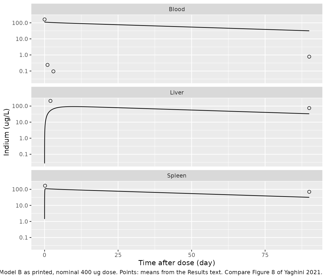
The paper’s Results text gives mean observed indium concentrations at several times, which are overlaid below. Neither model reproduces them.
Figure 5 (Model A, serum 0-24 h)
th_a <- exp(rxode2::rxode(mod_a)$theta[c("lcl", "lvc", "lq", "lvp")])
k10 <- th_a[["lcl"]] / th_a[["lvc"]]
k12_a <- th_a[["lq"]] / th_a[["lvc"]]
k21_a <- th_a[["lq"]] / th_a[["lvp"]]
lambda_a <- eigen(matrix(c(-(k10 + k12_a), k21_a, k12_a, -k21_a), 2, byrow = TRUE))$values
thalf_a_min <- sort(60 * log(2) / -lambda_a)
thalf_a_min
#> [1]  0.2012727 76.1585413
Table 1’s parameters give distribution and terminal half-lives of 0.2 and 76 min. Figure 5’s fitted line instead falls about 100-fold in the first hour (a half-life of about 8 min) and then about 4-fold between 2 and 24 h (about 12 h). Because the dose units are unknown, the second panel rescales the model profile to the observed 5-min mean so that only the shape is compared.
obs_serum <- tibble::tribble(
  ~time, ~conc,
  5 / 60, 162.48,
  20 / 60, 93.93,
  40 / 60, 10.36,
  24, 0.24
)
c5_a <- sim_a$Cc[which.min(abs(sim_a$time - 5 / 60))]
fig5 <- dplyr::bind_rows(
  sim_a |> dplyr::transmute(time, Cc, panel = "Nominal 400 ug dose"),
  sim_a |> dplyr::transmute(time, Cc = Cc * 162.48 / c5_a, panel = "Rescaled to the 5-min mean")
) |>
  dplyr::filter(time > 0)
ggplot(fig5, aes(time, Cc)) +
  geom_line() +
  geom_point(data = obs_serum, aes(time, conc), shape = 1, size = 2) +
  facet_wrap(~panel) +
  scale_y_log10() +
  coord_cartesian(ylim = c(0.01, 2e5)) +
  labs(
    x = "Time after dose (h)", y = "Serum indium (ug/L)",
    caption = "Lines: Model A as printed. Points: means from the Results text. Compare Figure 5 of Yaghini 2021."
  )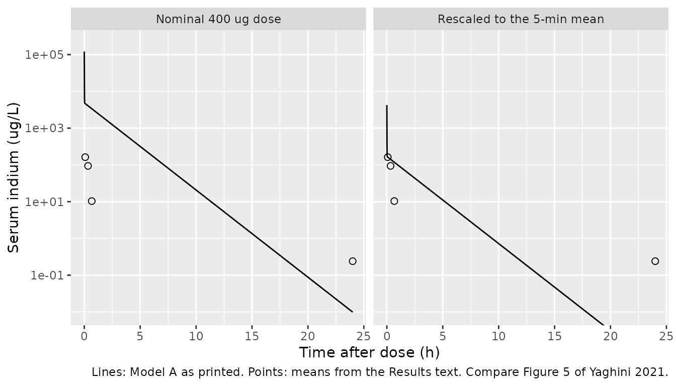
Figure 8 (Model B, blood, liver and spleen 0-90 days)
obs_organ <- tibble::tribble(
  ~time, ~conc, ~organ,
  5 / 60, 162.48, "Blood",
  24, 0.24, "Blood",
  72, 0.095, "Blood",
  90 * 24, 0.78, "Blood",
  48, 209.39, "Liver",
  90 * 24, 75.13, "Liver",
  4, 167.46, "Spleen",
  90 * 24, 69.98, "Spleen"
)
sim_b_long <- sim_b |>
  dplyr::select(time, Blood = Cc, Liver = Cliver, Spleen = Cspleen) |>
  tidyr::pivot_longer(-time, names_to = "organ", values_to = "conc") |>
  dplyr::filter(time > 0)
ggplot(sim_b_long, aes(time / 24, conc)) +
  geom_line() +
  geom_point(data = obs_organ, shape = 1, size = 2) +
  facet_wrap(~organ, ncol = 1) +
  scale_y_log10() +
  labs(
    x = "Time after dose (day)", y = "Indium (ug/L)",
    caption = "Lines: Model B as printed, nominal 400 ug dose. Points: means from the Results text. Compare Figure 8 of Yaghini 2021."
  )
pred_at <- function(sim, col, t) {
  sim[[col]][which.min(abs(sim$time - t))]
}
obs_organ |>
  dplyr::mutate(
    col = c(Blood = "Cc", Liver = "Cliver", Spleen = "Cspleen")[organ],
    predicted = mapply(function(cc, tt) pred_at(sim_b, cc, tt), col, time),
    ratio = predicted / conc
  ) |>
  dplyr::transmute(
    organ,
    time_h = round(time, 3),
    observed = conc,
    predicted = signif(predicted, 3),
    ratio = signif(ratio, 2)
  ) |>
  dplyr::rename(
    "Organ" = organ,
    "Time (h)" = time_h,
    "Observed mean (ug/L)" = observed,
    "Model B, 400 ug (ug/L)" = predicted,
    "Predicted / observed" = ratio
  ) |>
knitr::kable(caption = "Model B predictions at the times for which the Results text gives observed means.")| Organ | Time (h) | Observed mean (ug/L) | Model B, 400 ug (ug/L) | Predicted / observed |
|---|---|---|---|---|
| Blood | 0.083 | 162.480 | 117.0 | 0.72 |
| Blood | 24.000 | 0.240 | 108.0 | 450.00 |
| Blood | 72.000 | 0.095 | 103.0 | 1100.00 |
| Blood | 2160.000 | 0.780 | 31.8 | 41.00 |
| Liver | 48.000 | 209.390 | 52.2 | 0.25 |
| Liver | 2160.000 | 75.130 | 33.1 | 0.44 |
| Spleen | 4.000 | 167.460 | 105.0 | 0.63 |
| Spleen | 2160.000 | 69.980 | 31.8 | 0.45 |
At the nominal dose the spleen and late liver predictions are within
a few-fold of the observations, but blood stays near 100 ug/L for weeks,
40- to 1100-fold above the measured values. The structure forces this:
with uptake at Q/Vb and return at Q/VT, the
liver and spleen equilibrate at the blood concentration (tissue/blood
ratio of 1), while the data show tissue concentrations about 100-fold or
more above blood. No partition coefficient is reported.
PKNCA validation
nca_in <- dplyr::bind_rows(
  sim_a |> dplyr::transmute(id, time, Cc, treatment = "Model A (0-24 h)"),
  sim_b |> dplyr::transmute(id, time, Cc, treatment = "Model B (0-90 d)")
) |>
  dplyr::filter(!is.na(Cc))
stopifnot(all(nca_in$Cc >= -1e-6 * max(nca_in$Cc)))
nca_in <- nca_in |> dplyr::mutate(Cc = pmax(Cc, 0))

dose_df <- tibble::tibble(
  id = 1L, time = 0, amt = dose_ug,
  treatment = c("Model A (0-24 h)", "Model B (0-90 d)")
)
conc_obj <- PKNCA::PKNCAconc(nca_in, Cc ~ time | treatment + id)
dose_obj <- PKNCA::PKNCAdose(dose_df, amt ~ time | treatment + id, route = "intravascular")
intervals <- data.frame(
  start = 0, end = Inf,
  cmax = TRUE, aucinf.obs = TRUE, half.life = TRUE
)
nca_res <- PKNCA::pk.nca(PKNCA::PKNCAdata(conc_obj, dose_obj, intervals = intervals))
nca_wide <- as.data.frame(nca_res) |>
  dplyr::select(treatment, PPTESTCD, PPORRES) |>
  tidyr::pivot_wider(names_from = PPTESTCD, values_from = PPORRES)

# AUC0-inf must equal Dose / CL for a linear model with elimination from the
# sampled compartment.
auc_expected <- c(
  "Model A (0-24 h)" = dose_ug / 0.0416,
  "Model B (0-90 d)" = dose_ug / 0.0021
)
auc_err <- nca_wide$aucinf.obs / auc_expected[nca_wide$treatment] - 1
stopifnot(all(abs(auc_err) < 0.05))
The AUC0-inf identity holds to 0.16%.
Comparison against published half-lives
The paper reports a blood half-life for each model and no other NCA quantity.
published <- tibble::tribble(
  ~treatment, ~half.life,
  "Model A (0-24 h)", 28 / 60,
  "Model B (0-90 d)", 47.0 * 24
)
cmp <- nlmixr2lib::ncaComparisonTable(
  simulated = nca_res,
  reference = published,
  by = "treatment",
  units = c(half.life = "h"),
  tolerance_pct = 20
)
knitr::kable(cmp, caption = "Simulated terminal half-life vs. Table 1 / Table 2. * differs by >20%.")| NCA parameter | treatment | Reference | Simulated | % diff |
|---|---|---|---|---|
| t½ (h) | Model A (0-24 h) | 0.467 | 1.27 | +171.7%* |
| t½ (h) | Model B (0-90 d) | 1130 | 1240 | +9.6% |
Model B’s simulated terminal half-life (51.5 days) is the slowest
eigenvalue of the three-compartment system and sits close to the printed
47 days, which is log(2)/ke. Model A’s simulated terminal
half-life (76.1 min) does not match the printed 28 min; no combination
of the Table 1 values gives 28 min.
Assumptions and deviations
-
Neither model reproduces the paper’s own figures.
The maintainers packaged both tables as printed and kept the mismatch
visible above rather than adjusting any value. In Model A, the Table 1
parameters give half-lives of about 0.2 and 76 min; Figure 5 needs
roughly 8 min and 12 h. A search over CL/Q and V1/V2 swaps and minute,
hour and day rescalings of CL and Q found no reading that reproduces
Figure 5. In Model B, blood cannot fall from about 160 to 0.3 ug/L
within 2 h when the total blood exit rate
k12 + k13 + keis 0.048 1/h, and the structure without a partition coefficient holds tissue and blood at equal concentrations. -
Model B equations are written on amounts. Eqs
(3)-(5) are printed on concentrations
C1-C3but use theQ/Vb,Q/VTrate constants of eqs (6)-(10), which give a mass-balanced system only when the states are amounts (NONMEM ADVAN6 integrates amounts). The concentration form as printed would put equilibrium tissue concentrations atVT/Vbtimes blood (26-fold below blood in the liver, 15-fold in the spleen), further from Figure 8. -
Liver is compartment 2 and spleen compartment 3,
following eqs (4)-(5), the Table 2 tissue column, the Figure 1B caption
and the data (the spleen peaks at 4 h, consistent with the fast
k31; the liver at day 2, consistent with the slowk21). The Table 2 footnote’s ‘K21 = equilibration rate constant from spleen to blood’ swaps the organs and was not followed. -
The spleen half-life is printed as 1.0 day but
log(2)/K31is 0.95 h. - VT1 + VT2 = 0.35 L exceeds Vtot - Vb = 0.24 L, so the volume fractions FV1 and FV2 of the Figure 1B caption sum to 1.46. Vb = 3.41 L and Vtot = 3.65 L are also far larger than a mouse; they are apparent volumes on an unstated dose scale.
- Dose units are not stated. The dose is 20 mg/kg of quantum dot; the analyte is indium, whose fraction is unreported, and no body weights are given. The vignette uses a nominal 400 ug.
-
Model A residual error. Table 1 prints
‘Proportional error 0.0686’ and ‘Additive error (ng/L) 0.05 (38%)’
without a scale. The maintainers read both as NONMEM
$SIGMAvariances because Methods eq (2) defines epsilon by its variance sigma^2, and because the replicate spread around the Figure 5 curve (roughly 20% on the log scale, read off the figure) is closer to the variance reading’s SD of 26% than to the 6.9% of the SD reading. The additive term is printed in ng/L while concentrations are in ug/L, so the SD is 0.000224 ug/L and effectively zero. The ‘(38%)’ is not explained. -
Model B residual error is described as
‘proportional and additive’, but no values are printed. All six residual
parameters are
fixed(0)placeholders. - No correction notice for this article was found on 2026-10-16. The supplement contains only haematology and clinical-chemistry figures from the rat toxicology arm.