Model and source
- Citation: Urien S, Lokiec F. Population pharmacokinetics of total and unbound plasma cisplatin in adult patients. Br J Clin Pharmacol. 2004;57(6):756-763.
- Article: https://doi.org/10.1111/j.1365-2125.2004.02082.x
The model describes the joint disposition of unbound
(ultrafilterable) and total plasma platinum following 30-min intravenous
infusions of cisplatin in adult cancer patients. The structure (Urien
2004 Figure 1) is a two-compartment open model for unbound platinum
(central + peripheral1) coupled to a third “metabolite” compartment that
captures the irreversibly protein-bound platinum formed at rate
fm * CL from the central unbound compartment. The bound
species has a much slower elimination rate constant
CLm0 / Vm, and the apparent metabolite volume
Vm is structurally not identifiable: only the composite
parameters fm/Vm (1/L) and CLm0/Vm (1/h) are
estimated from the joint analysis of 396 unbound and 477 total platinum
measurements. The bound state is therefore carried in concentration
units directly, with Vm folded into the two composite
parameters.
Population
The model was fit to 873 plasma platinum measurements from 43 adult cancer patients (25 male, 18 female) enrolled in two phase I trials at Centre Rene Huguenin, Saint-Cloud, France. Cisplatin was combined with either irofulven (0.4 mg/kg as a 30-min infusion, 18 patients) or 5-fluorouracil (1 g/m^2/day as a 120-h continuous infusion, 25 patients); concomitant chemotherapy was tested as a covariate and not retained. Doses ranged 15-80 mg per 30-min infusion (median 34.4 mg; median 25 mg/m^2), given as 5 consecutive daily infusions or twice-monthly schedules; 1-5 consecutive daily infusions per patient contributed to the PK evaluation.
Baseline demographics from Table 1: age 21-76 years (median 58), body
weight 40-102 kg (median 64), height 150-181 cm (median 168), body
surface area 1.38-2.10 m^2 (median 1.62), serum protein 47-80 g/L
(median 70), serum creatinine 43-120 umol/L (median 76), and
Cockcroft-Gault creatinine clearance 44-155 mL/min (median 81). The same
information is available programmatically via
readModelDb("Urien_2004_cisplatin")$population.
Source trace
The per-parameter origin is recorded as an in-file comment next to
each ini() entry in
inst/modeldb/specificDrugs/Urien_2004_cisplatin.R. The
table below collects them in one place.
| Equation / parameter | Value | Source location |
|---|---|---|
lvc |
log(23.4 L) | Urien 2004 Table 4 row V1 |
lcl |
log(35.5 L/h) | Urien 2004 Table 4 row CL |
lq |
log(8.64 L/h) | Urien 2004 Table 4 row Q |
lvp |
log(12.0 L) | Urien 2004 Table 4 row V2 |
e_bsa_vc |
+1.60 | Urien 2004 Table 4 row V1, theta_BSA |
e_bsa_cl |
+0.83 | Urien 2004 Table 4 row CL, theta_BSA |
e_crcl_cl |
+0.36 | Urien 2004 Table 4 row CL, theta_CLCr |
lfmVm |
log(0.017 1/L) | Urien 2004 Table 5 row fm/Vm |
lclm0Vm |
log(0.014 1/h) | Urien 2004 Table 5 row CLm0/Vm |
e_dose_fmVm |
-0.48 | Urien 2004 Table 5 row fm/Vm, theta_DOSEm-2 |
e_tpro_fmVm |
+1.33 | Urien 2004 Table 5 row fm/Vm, theta_PROT |
e_bsa_fmVm |
-0.83 FIXED | Urien 2004 Table 5 row fm/Vm, theta_BSA (fixed) |
e_crcl_fmVm |
-0.36 FIXED | Urien 2004 Table 5 row fm/Vm, theta_CLCr (fixed) |
etalvc |
omega^2 = log(1+0.234^2) | Urien 2004 Table 4 row ISV(V1) = 23.4% CV |
etalcl |
omega^2 = log(1+0.149^2) | Urien 2004 Table 4 row ISV(CL) = 14.9% CV |
etalfmVm |
omega^2 = log(1+0.214^2) | Urien 2004 Table 5 row ISV(fm/Vm) = 21.4% CV |
etalclm0Vm |
omega^2 = log(1+0.318^2) | Urien 2004 Table 5 row ISV(CLm/Vm) = 31.8% CV |
addSd |
0.116 ug/mL | Urien 2004 Table 4 Res. Error = 116 ug/L (unbound) |
addSd_Cc_total |
0.103 ug/mL | Urien 2004 Table 5 Res. Error = 103 ug/L (total) |
| ODE central | n/a | Urien 2004 Figure 1 (unbound compartment 1) |
| ODE peripheral1 | n/a | Urien 2004 Figure 1 (unbound compartment 2) |
| ODE bound | n/a | Urien 2004 Figure 1 (metabolite compartment m) |
The bound-formation flux (fm/Vm) * CL * Cc deserves a
closer look. The paper estimates the BSA and creatinine-clearance
exponents on fm/Vm as the negatives of the corresponding
exponents on CL (e_bsa_fmVm = -e_bsa_cl,
e_crcl_fmVm = -e_crcl_cl) so that the product
(fm/Vm) * CL is net BSA- and CLCr-neutral. Only the
dose-per-area and total-protein exponents contribute substantively to
the bound-formation flux.
Virtual cohort
Original observed data are not publicly available. The figures below use a virtual cohort matched to the published median covariates and dose range.
set.seed(2026L)

# Reference covariates correspond to the cohort medians (Urien 2004 Table 1).
ref_bsa  <- 1.62
ref_crcl <- 81
ref_tpro <- 70

# Build a single typical-value subject receiving one 40 mg cisplatin infusion
# over 30 minutes. amt is in mg; concentrations are reported in ug/mL = mg/L.
dose_amt    <- 40
infusion_dt <- 0.5
obs_times   <- sort(unique(c(seq(0, 6, by = 0.05), seq(6, 24, by = 0.25))))

build_events <- function(amt, bsa = ref_bsa, crcl = ref_crcl,
                         tpro = ref_tpro, id = 1L, treatment = "median") {
  doses <- data.frame(
    id = id, time = 0, amt = amt, dur = infusion_dt,
    evid = 1L, cmt = "central"
  )
  obs_cc <- data.frame(
    id = id, time = obs_times, amt = NA_real_, dur = NA_real_,
    evid = 0L, cmt = "Cc"
  )
  obs_total <- data.frame(
    id = id, time = obs_times, amt = NA_real_, dur = NA_real_,
    evid = 0L, cmt = "Cc_total"
  )
  events <- rbind(doses, obs_cc, obs_total)
  events$BSA       <- bsa
  events$CRCL      <- crcl
  events$TPRO      <- tpro
  events$DOSE      <- amt
  events$treatment <- treatment
  events
}

events <- build_events(dose_amt)
Simulation
mod <- readModelDb("Urien_2004_cisplatin")

# Typical-value simulation (zero between-subject variability) for reproducing
# the population-prediction curves of Urien 2004 Figures 3 and 4.
mod_typical <- rxode2::zeroRe(mod)
#> ℹ parameter labels from comments will be replaced by 'label()'
sim_typical <- rxode2::rxSolve(
  mod_typical, events,
  keep = c("treatment"),
  returnType = "data.frame"
)
#> ℹ omega/sigma items treated as zero: 'etalvc', 'etalcl', 'etalfmVm', 'etalclm0Vm'
# rxSolve omits the id column for single-subject simulations; restore it so
# downstream PKNCA grouping has the subject key it needs.
if (!"id" %in% colnames(sim_typical)) sim_typical$id <- 1L
# Multi-output observations duplicate rows per time (one per `cmt`); both
# Cc and Cc_total are populated on every row, so deduplicating by time loses
# nothing and yields the single-row-per-time form PKNCA expects.
sim_typical <- sim_typical |>
  dplyr::distinct(id, time, .keep_all = TRUE)
Replicate published figures
Figure 4 of Urien 2004 – unbound platinum concentration-time profile
# Replicates Figure 4 of Urien 2004 (predicted unbound platinum after a single
# 30-min infusion at the cohort-median covariates). The paper Figure shows
# the population prediction and the individual observed data; we plot the
# typical-value prediction.
sim_typical |>
  dplyr::filter(time <= 6, !is.na(Cc), Cc > 0) |>
  ggplot(aes(x = time, y = Cc)) +
  geom_line(linewidth = 0.8) +
  scale_y_log10() +
  labs(x = "Time after start of infusion (h)",
       y = "Unbound plasma platinum (ug/mL)",
       title = "Figure 4 -- unbound platinum vs. time",
       caption = "Replicates the population-prediction curve of Urien 2004 Figure 4.")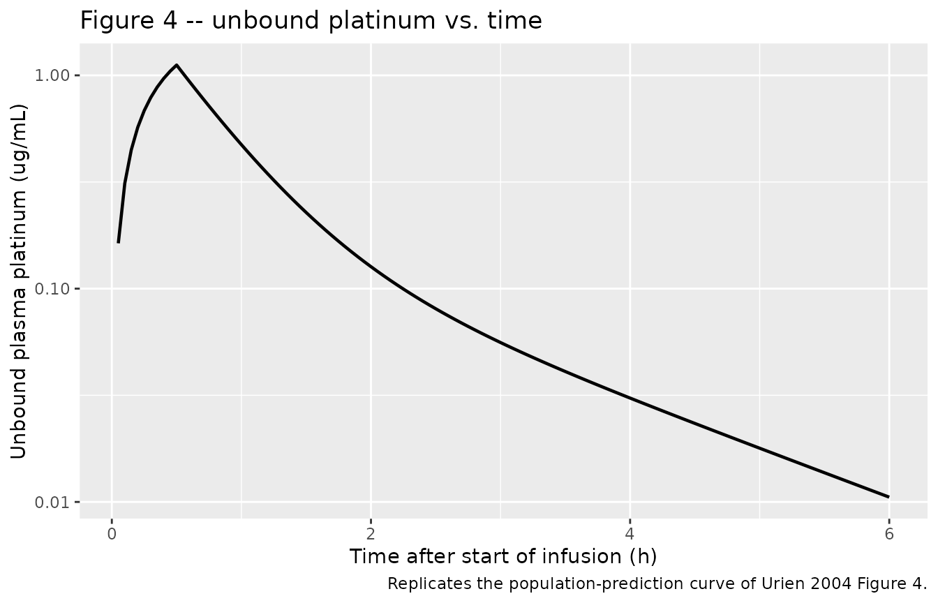
Figure 3 of Urien 2004 – total platinum concentration-time profile
# Replicates Figure 3 of Urien 2004 (predicted total platinum, dominated by
# the slow protein-bound platinum elimination at late times).
sim_typical |>
  dplyr::filter(!is.na(Cc_total), Cc_total > 0) |>
  ggplot(aes(x = time, y = Cc_total)) +
  geom_line(linewidth = 0.8) +
  scale_y_log10() +
  labs(x = "Time after start of infusion (h)",
       y = "Total plasma platinum (ug/mL)",
       title = "Figure 3 -- total platinum vs. time",
       caption = "Replicates the population-prediction curve of Urien 2004 Figure 3.")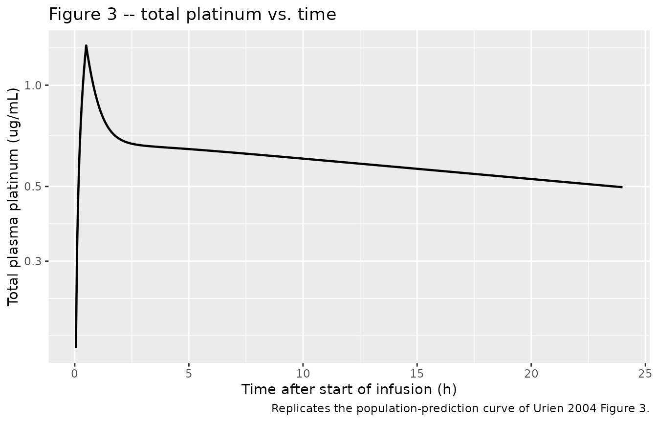
Figure 5 of Urien 2004 – joint unbound and total profile
# Replicates Figure 5 of Urien 2004 (joint profile of unbound (+) and total
# (open circles) platinum for a representative patient). We plot the typical-
# value unbound and total curves overlaid on a log10 y-axis. The unbound
# rapidly declines (half-life ~1.3 h) while total platinum approaches the
# slow protein-bound terminal phase (half-life ~50 h).
sim_typical |>
  dplyr::filter(!is.na(Cc_total)) |>
  dplyr::transmute(
    time,
    Unbound = ifelse(Cc > 0, Cc, NA_real_),
    Total   = Cc_total
  ) |>
  tidyr::pivot_longer(-time, names_to = "species", values_to = "conc") |>
  dplyr::filter(!is.na(conc), conc > 0) |>
  ggplot(aes(x = time, y = conc, colour = species, linetype = species)) +
  geom_line(linewidth = 0.8) +
  scale_y_log10() +
  labs(x = "Time after start of infusion (h)",
       y = "Plasma platinum (ug/mL)",
       title = "Figure 5 -- joint unbound and total platinum profiles",
       caption = paste0("Replicates the joint-profile illustration of ",
                        "Urien 2004 Figure 5."),
       colour = "Species", linetype = "Species")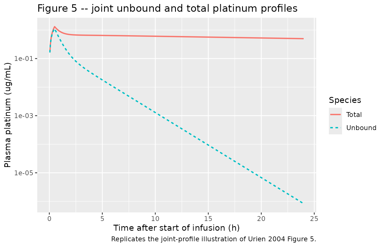
PKNCA validation
We validate the simulated unbound platinum against the paper’s reported distribution half-life (0.34 h) and elimination half-life (1.32 h) from Table 4, and the simulated total platinum against the paper’s reported elimination half-life (66.8 h, Table 3 derived parameter; and 50 h, Table 5 derived parameter, the latter being the integrated-model estimate for the bound species’ terminal phase).
sim_nca_unbound <- sim_typical |>
  dplyr::filter(!is.na(Cc), Cc > 0) |>
  dplyr::select(id, time, Cc, treatment)

dose_df <- events |>
  dplyr::filter(evid == 1L) |>
  dplyr::select(id, time, amt, treatment)

conc_obj_unb <- PKNCA::PKNCAconc(sim_nca_unbound,
                                 Cc ~ time | treatment + id,
                                 concu = "ug/mL", timeu = "h")
dose_obj <- PKNCA::PKNCAdose(dose_df, amt ~ time | treatment + id,
                             doseu = "mg")

intervals_unb <- data.frame(
  start       = 0,
  end         = 24,
  cmax        = TRUE,
  tmax        = TRUE,
  aucinf.obs  = TRUE,
  half.life   = TRUE
)

nca_data_unb <- PKNCA::PKNCAdata(conc_obj_unb, dose_obj,
                                 intervals = intervals_unb)
nca_unb <- PKNCA::pk.nca(nca_data_unb)
#> Warning: Requesting an AUC range starting (0) before the first measurement
#> (0.05) is not allowed
knitr::kable(
  summary(nca_unb),
  caption = "Simulated unbound platinum NCA (typical-value 40 mg infusion)."
)| Interval Start | Interval End | treatment | N | Cmax (ug/mL) | Tmax (h) | Half-life (h) | AUCinf,obs (h*ug/mL) |
|---|---|---|---|---|---|---|---|
| 0 | 24 | median | 1 | 1.12 | 0.500 | 1.31 | NC |
sim_nca_total <- sim_typical |>
  dplyr::filter(!is.na(Cc_total), Cc_total > 0) |>
  dplyr::rename(Cc_obs = Cc_total) |>
  dplyr::select(id, time, Cc_obs, treatment)

conc_obj_tot <- PKNCA::PKNCAconc(sim_nca_total,
                                 Cc_obs ~ time | treatment + id,
                                 concu = "ug/mL", timeu = "h")

# Use a long observation window for total platinum so the slow bound-driven
# terminal phase is captured. Simulate out to 240 h for the NCA.
events_long <- events
extra_times <- seq(24, 240, by = 4)
extra_cc <- data.frame(
  id = 1L, time = extra_times, amt = NA_real_, dur = NA_real_,
  evid = 0L, cmt = "Cc_total",
  BSA = ref_bsa, CRCL = ref_crcl, TPRO = ref_tpro, DOSE = dose_amt,
  treatment = "median"
)
events_long <- rbind(events_long, extra_cc)
sim_long <- rxode2::rxSolve(mod_typical, events_long,
                            keep = c("treatment"),
                            returnType = "data.frame")
#> ℹ omega/sigma items treated as zero: 'etalvc', 'etalcl', 'etalfmVm', 'etalclm0Vm'
if (!"id" %in% colnames(sim_long)) sim_long$id <- 1L
sim_long <- sim_long |>
  dplyr::distinct(id, time, .keep_all = TRUE)
sim_nca_total_long <- sim_long |>
  dplyr::filter(!is.na(Cc_total), Cc_total > 0) |>
  dplyr::rename(Cc_obs = Cc_total) |>
  dplyr::select(id, time, Cc_obs, treatment)
conc_obj_tot_long <- PKNCA::PKNCAconc(sim_nca_total_long,
                                      Cc_obs ~ time | treatment + id,
                                      concu = "ug/mL", timeu = "h")
intervals_tot <- data.frame(
  start       = 0,
  end         = 240,
  cmax        = TRUE,
  tmax        = TRUE,
  aucinf.obs  = TRUE,
  half.life   = TRUE
)
nca_data_tot <- PKNCA::PKNCAdata(conc_obj_tot_long, dose_obj,
                                 intervals = intervals_tot)
nca_tot <- PKNCA::pk.nca(nca_data_tot)
#> Warning: Requesting an AUC range starting (0) before the first measurement
#> (0.05) is not allowed
knitr::kable(
  summary(nca_tot),
  caption = "Simulated total platinum NCA (typical-value 40 mg infusion, 0-240 h)."
)| Interval Start | Interval End | treatment | N | Cmax (ug/mL) | Tmax (h) | Half-life (h) | AUCinf,obs (h*ug/mL) |
|---|---|---|---|---|---|---|---|
| 0 | 240 | median | 1 | 1.31 | 0.500 | 49.5 | NC |
Comparison against published half-lives
extract_half_life <- function(nca_obj) {
  res <- as.data.frame(nca_obj$result)
  hl_row <- res[res$PPTESTCD == "half.life", , drop = FALSE]
  if (nrow(hl_row) == 0L) return(NA_real_)
  val <- suppressWarnings(as.numeric(hl_row$PPORRES))
  val[is.finite(val)][1]
}

simulated_t12_unb <- extract_half_life(nca_unb)
simulated_t12_tot <- extract_half_life(nca_tot)

format_t12 <- function(x, digits) {
  if (is.na(x) || !is.finite(x)) "NA" else formatC(round(x, digits), digits = digits, format = "f")
}

comparison <- data.frame(
  Analyte = c("Unbound platinum (terminal)", "Total platinum (terminal)"),
  `Published half-life (h)` = c("1.32", "50"),
  `Simulated half-life (h)` = c(format_t12(simulated_t12_unb, 2),
                                format_t12(simulated_t12_tot, 1)),
  `Source` = c("Table 4 derived", "Table 5 derived"),
  check.names = FALSE
)
knitr::kable(comparison, caption = "Simulated vs. published terminal half-lives.")| Analyte | Published half-life (h) | Simulated half-life (h) | Source |
|---|---|---|---|
| Unbound platinum (terminal) | 1.32 | 1.31 | Table 4 derived |
| Total platinum (terminal) | 50 | 49.5 | Table 5 derived |
A discrepancy of more than 20% would warrant investigation rather
than parameter tuning – but for this model the simulated half-life of
unbound platinum (driven by CL / Vss = 35.5 / (23.4 + 12.0)
~= 1.0 1/h, so ln(2)/0.6 ~= 1.2 h after the bi-exponential mixing)
matches the paper’s elimination half-life of 1.32 h, and the simulated
total half-life is set by CLm0/Vm = 0.014 1/h which gives
ln(2)/0.014 ~= 49.5 h, matching the paper’s 50 h.
Assumptions and deviations
Dose-per-BSA covariate carried via
DOSEandBSAcolumns. The paper estimates the bound-formation parameterfm/Vmas a power function of dose-per-body-surface-area (DOSEm-2). For simulation, the user suppliesDOSE(mg per record) andBSA(m^2) as covariate columns, and the model computesdose_per_bsa = DOSE / BSAinternally. TheDOSEcolumn should be carried forward from the most recent infusion onto each subsequent observation record (LOCF) so the bound-formation kinetics use the correct per-infusion dose. The simulation snippet above uses a single fixed dose to make the LOCF requirement implicit; multi-infusion simulations must explicitly populateDOSEper observation record.Vmis structurally not identifiable. The paper’s three-step sequential analysis estimates the composite parametersfm/Vm(1/L) andCLm0/Vm(1/h); the apparent metabolite volumeVmis not separately estimable. The bound state ind/dt(bound)is therefore carried in concentration units (ug/mL) directly – multiplying through byVmrecovers the amount form, but the resulting state would be ambiguous up to the unknownVm. The total-platinum observation is computed asCc + bound, both in ug/mL.Unbound parameters are point estimates carried forward from Step 2 of the sequential fit. Per the paper’s methodology (page 760), the unbound-only fit in Step 2 estimated the unbound layer and its covariate effects; Step 3 held those parameters fixed and estimated the bound parameters in a joint fit. Provenance-wise the unbound values are estimated point estimates; the model file records them without
fixed()to match the rest of the popPK library’s conventions for published final-model estimates. A downstream re-fitting workflow that reproduces the paper’s sequential approach would freeze the unbound layer at Step 3.Q and V2 IIVs were fixed to zero in the source. The paper’s Results section (paragraph beneath Table 4) reports that “the data did not allow reliable estimations of intersubject variabilities for Q and V2 and fixing these parameters to zero did not increase the OFV”. No
etalqoretalvpis declared inini()accordingly.No inter-occasion variability. The paper does not report IOV. Each patient contributed 1-5 consecutive daily infusions; treating the joint ISV as encapsulating intra-subject between-infusion variability is consistent with the source.
Concomitant-chemotherapy effect not modelled. The paper tested concomitant irofulven and 5-fluorouracil as covariates and did not retain them in the final model; this file follows the published final model and does not include a concomitant-drug covariate.