Tominersen (Yamamoto 2023) • nlmixr2lib

Model and source

Citation: Yamamoto Y, Sanwald Ducray P, Bjornsson M, Smart K, Grimsey P, Vatakuti S, Portron A, Massonnet B, Norris DA, Silber Baumann HE. Development of a population pharmacokinetic model to characterize the pharmacokinetics of intrathecally administered tominersen in cerebrospinal fluid and plasma. CPT Pharmacometrics Syst Pharmacol. 2023;12(9):1213-1226. doi:10.1002/psp4.13001
Description: Six-compartment population PK model for tominersen (2’-O-methoxyethyl antisense oligonucleotide targeting huntingtin mRNA) following intrathecal lumbar-puncture administration in adults with Huntington’s disease (Yamamoto 2023). Two coupled three-compartment subsystems: the intrathecal bolus enters the central CSF compartment, which exchanges with two CNS-tissue compartments and drains unidirectionally into the plasma central compartment via CL_CSF (bioavailability F1 and F2 both fixed to 1); the plasma central compartment has two peripheral compartments and first-order elimination. Baseline CSF total protein, age, and antidrug antibodies are covariates on CL_CSF; body weight is an allometric power covariate on all plasma clearances and volumes, and antidrug antibodies and female sex are covariates on plasma CL. Residual error is additive on the log scale (lognormal) for both CSF and plasma, each with interindividual variability on the residual magnitude.
Article: https://doi.org/10.1002/psp4.13001
Appendix S1 (final NONMEM control stream plus Tables S1-S3 and Figure S1) is the supporting information for the same DOI.

Tominersen is a 2’-O-methoxyethyl-modified antisense oligonucleotide that lowers huntingtin mRNA. It is given as an intrathecal bolus, so the cerebrospinal fluid (CSF) is both the dosing site and the compartment closest to the target tissue; plasma exposure arises only from drug that has already transferred out of the CSF. The model therefore couples two three-compartment subsystems in series rather than treating CSF as a peripheral compartment hanging off plasma.

Population

The model was built on pooled data from five clinical studies in adults with early manifest or manifest Huntington’s disease: the phase I/IIa study (NCT02519036), its open-label extension (NCT03342053), GEN-PEAK (NCT04000594), GENERATION HD1 (NCT03761849), and GEN-EXTEND (NCT03842969). A total of 750 participants contributed 6302 CSF and 5454 plasma concentrations (Yamamoto 2023 Table 1). Doses ranged from 10 to 120 mg given every 4, 8, or 16 weeks, for up to 25 months; almost every dose was given by lumbar puncture (L3-L4 in 60.7% to 67.6% of administrations, Table S2), while GEN-PEAK used an indwelling intrathecal catheter to enable rich 72-hour CSF sampling.

Baseline demographics (Table S1) span 40.1 to 116 kg body weight (study medians 69.1 to 75.3 kg), 25 to 66 years of age (study medians 46 to 50), and 0 to 15.5 g/L CSF total protein (study medians 0.305 to 0.372 g/L); 350 of the 750 participants (46.7%) were women. Creatinine clearance spanned 50.6 to 168.7 mL/min and was not retained as a covariate. ADA status was recorded per concentration record (Tables S3A and S3B) and was not measured at all in the phase I/IIa study or GEN-PEAK. Four percent of CSF and 19% of plasma samples were below the limit of quantification and were excluded from the fit.

The same information is available programmatically via the model’s population metadata (readModelDb("Yamamoto_2023_tominersen")()$population).

Source trace

The per-parameter origin is recorded as an in-file comment next to each ini() entry in inst/modeldb/specificDrugs/Yamamoto_2023_tominersen.R. The table below collects them in one place for review. “Appendix S1” refers to the final NONMEM control stream reproduced in the supporting information.

Because the CSF subsystem was fitted first and then held fixed while the plasma subsystem was fitted, the control stream carries the CSF parameters as FIX values – these are the CSF fit’s final estimates, at greater precision than Table 2’s three significant figures. The plasma parameters were the ones being estimated in that run, so the control stream shows only their initial values and the final plasma estimates come from Table 2.

Equation / parameter	Value	Source location
`lcl_csf` (CL_CSF)	0.0176577 L/h	Appendix S1 `$THETA(3)` FIX; Table 2 0.0177, RSE 7.96%
`lvcsf` (V1,CSF)	0.0436042 L	Appendix S1 `$THETA(4)` FIX; Table 2 0.0436, RSE 33.1%
`lqcsf` (Q2,CSF)	0.00982466 L/h	Appendix S1 `$THETA(5)` FIX; Table 2 0.00982, RSE 27.3%
`lvcns` (V2,CSF)	0.0517384 L	Appendix S1 `$THETA(6)` FIX; Table 2 0.0517, RSE 11.8%
`lqcsf2` (Q3,CSF)	1.20953e-05 L/h	Appendix S1 `$THETA(7)` FIX; Table 2 0.0000121, RSE 15.7%
`lvcns2` (V3,CSF)	0.0117556 L	Appendix S1 `$THETA(8)` FIX; Table 2 0.0118, RSE 15.8%
`lcl` (CL_plasma)	10.7 L/h	Table 2, RSE 3.30% (Appendix S1 `$THETA(9)` initial 9.95883)
`lvc` (V1,plasma)	41.0 L	Table 2, RSE 2.88% (Appendix S1 `$THETA(10)` initial 41.1879)
`lq` (Q2,plasma)	13.4 L/h	Table 2, RSE 7.98% (Appendix S1 `$THETA(11)` initial 14.2579)
`lvp` (V2,plasma)	283 L	Table 2, RSE 6.15% (Appendix S1 `$THETA(12)` initial 273.266)
`lq2` (Q3,plasma)	0.267 L/h	Table 2, RSE 4.84% (Appendix S1 `$THETA(13)` initial 0.276129)
`lvp2` (V3,plasma)	613 L	Table 2, RSE 6.35% (Appendix S1 `$THETA(14)` initial 619.497)
`e_tpcsf_cl_csf`	-0.539797	Appendix S1 `$THETA(15)` FIX; Table 2 -0.540, RSE 11.2%
`e_ada_cl_csf`	-0.100697	Appendix S1 `$THETA(16)` FIX; Table 2 -0.101, RSE 6.89%
`e_age_cl_csf`	-0.005498	Appendix S1 `$THETA(17)` FIX; Table 2 -0.00550, RSE 12.8%
`e_wt_cl` (BW_CLs)	0.687	Table 2, RSE 2.60% (Appendix S1 `$THETA(1)` initial 1.08182)
`e_wt_vc` (BW_Vs)	0.866	Table 2, RSE 1.54% (Appendix S1 `$THETA(2)` initial 0.913675)
`e_ada_cl`	-0.673	Table 2, RSE 0.639% (Appendix S1 `$THETA(18)` initial -0.672001)
`e_sexf_cl`	-0.186	Table 2, RSE 12.1% (Appendix S1 `$THETA(19)` initial -0.001)
`etalcl_csf`	0.0273094	Appendix S1 `$OMEGA(2)` FIX; Table 2 IIV on CL_CSF 16.5%
`etalvcsf`	0.312055	Appendix S1 `$OMEGA(3)` FIX; Table 2 IIV on V1,CSF 55.9%
`etalqcsf`	0.199008	Appendix S1 `$OMEGA(4)` FIX; Table 2 IIV on Q2,CSF 44.6%
`etalcl`	0.082944	Table 2 IIV on CL_plasma 28.8% (= 0.288^2)
`etalq`	5.7121	Table 2 IIV on Q2,plasma 239% (= 2.39^2)
`etalvp`	0.416025	Table 2 IIV on V2,plasma 64.5% (= 0.645^2)
`etalvp2`	0.367236	Table 2 IIV on V3,plasma 60.6% (= 0.606^2)
`etaexpSd_Ccsf`	0.214278	Appendix S1 `$OMEGA(1)` FIX; Table 2 IIV RUV CSF 46.3%
`etaexpSd`	0.0841	Table 2 IIV RUV plasma 29.0% (= 0.29^2)
`expSd_Ccsf`	sqrt(0.0975477)	Appendix S1 `$SIGMA(1)` FIX; Table 2 RUV CSF 31.2%
`expSd`	0.536	Table 2 RUV plasma 53.6% (Appendix S1 `$SIGMA(2)` initial 0.291491)
Zero IIV on V2,CSF / Q3,CSF / V3,CSF / V1,plasma / Q3,plasma	0	Appendix S1 `$OMEGA` 5, 6, 7, 9, 12 all `0 FIX`
Exponential (centered) continuous covariate form	n/a	Equation 2; Appendix S1 `$PK` `EXP(THETA*(COV - ref))`
Fractional-difference categorical covariate form	n/a	Equation 2; Appendix S1 `$PK` `1 + THETA`
Allometric power body-weight form, reference 75 kg	n/a	Appendix S1 `$PK` `(WT/75)**THETA`
CSF total-protein reference 0.35 g/L, age reference 49 y	n/a	Appendix S1 `$PK`; corroborated by the Figure 5 legend
CSF total-protein guard above 2 g/L	n/a	Appendix S1 `$PK` `IF(TPCSF.GT.2) CLCTPCSF=1`
Micro-constants K14, K12, K21, K13, K31, K40, K45, K54, K46, K64	n/a	Appendix S1 `$PK`
Six-compartment ODE system	n/a	Figure 3; Appendix S1 `$MODEL` / `$DES`
`/1000` concentration scaling (mg amounts to ng/mL)	n/a	Appendix S1 `$PK` `S1 = VC1/1000`, `S4 = V1/1000`
F1 = F2 = 1 (fixed)	1	Table 2; Methods “Disposition models for tominersen in CSF and plasma”
Additive residual error on log-transformed concentrations, with per-subject exp(eta) on the residual SD	n/a	Methods “Residual error”; Appendix S1 `$ERROR` `Y = IPRED + EPS(n)*EXP(ETA(k))`

Virtual cohort

Original observed data are not publicly available. The simulations below use virtual populations whose covariate distributions approximate the published trial demographics (Table S1), and typical-covariate scenarios matching the settings stated in the Figure 5 legend: ADA-negative, male, 75 kg, CSF total protein 0.35 g/L, age 49 years.

Observation rows use the ODE state csf as cmt together with dvid = 1L. rxode2 returns both algebraic observables (Ccsf and Cc) as columns on those rows, so a single observation row per time point covers both matrices.

set.seed(20260730)

week  <- 7 * 24          # hours per week
q16w  <- 16 * week       # Q16W dosing interval (h)
n_arm <- 200L            # subjects per dose arm (the cap)
eta_seed <- 4242L        # reused per arm so the dose arms are paired

doses <- c(30, 60, 90, 120)

# Typical-covariate settings from the Figure 5 legend.
tv_cov <- list(WT = 75, AGE = 49, SEXF = 0, ADA_POS = 0, CSF_TPRO = 0.35)

# Build an event table: one intrathecal bolus into `csf` (optionally repeated
# via ii/addl) plus observation rows on the same compartment.
make_events <- function(ids, dose, obs_times, covs, label,
                        ii = 0, addl = 0L) {
  dose_rows <- tibble(
    id = ids, time = 0, amt = dose, cmt = "csf", evid = 1L,
    ii = ii, addl = addl, dvid = NA_integer_
  )
  obs_rows <- tidyr::expand_grid(id = ids, time = obs_times) |>
    mutate(amt = NA_real_, cmt = "csf", evid = 0L,
           ii = 0, addl = 0L, dvid = 1L)
  bind_rows(dose_rows, obs_rows) |>
    left_join(covs, by = "id") |>
    mutate(regimen = label) |>
    arrange(id, time, desc(evid))
}

# Covariate marginals. Means and SDs are the GENERATION HD1 v.5 column of
# Table S1 (the largest contributing cohort, n = 518); each draw is truncated
# to the pooled analysis set's observed minimum and maximum.
sample_covs <- function(ids) {
  n <- length(ids)
  tibble(
    id       = ids,
    WT       = pmin(pmax(rnorm(n, 71.7, 13.3), 40.1), 116),
    AGE      = pmin(pmax(rnorm(n, 47.6, 9.47), 25), 66),
    CSF_TPRO = pmin(pmax(rnorm(n, 0.334, 0.113), 0.10), 1.0),
    SEXF     = rbinom(n, 1L, 0.467),   # Table S1: 350/750 women
    ADA_POS  = rbinom(n, 1L, 0.121)    # Table S3B: 12.1% of CSF records
  )
}

# ---- Cohort 1: population VPC, 30/60/90/120 mg Q16W for 1.5 years ----------
# Five Q16W doses (weeks 0, 16, 32, 48, 64); the steady-state trough is read at
# the end of the fifth interval (week 80), matching the paper's 1.5-year window.
#
# The four dose arms are deliberately PAIRED: one covariate draw is reused for
# every arm, and the eta seed is reset before each arm's solve, so subject k is
# the same virtual person at every dose. Because the model is linear, this makes
# the dose-response exactly proportional and removes the between-arm Monte Carlo
# noise that would otherwise swamp the plasma medians (Q2,plasma carries a 239%
# IIV). The proportionality is asserted after the solve.
obs_vpc <- sort(unique(c(seq(0, 5 * q16w, by = week), 5 * q16w)))

cov_pop <- sample_covs(seq_len(n_arm))

cohort_vpc <- bind_rows(lapply(doses, function(d) {
  make_events(seq_len(n_arm), d, obs_vpc, cov_pop,
              label = paste0(d, " mg Q16W"),
              ii = q16w, addl = 4L)
}))

# ---- Cohort 2: covariate scenarios at 120 mg Q16W (Figure 5c,d) ------------
scenarios <- tibble(
  id       = 1L:6L,
  scenario = c("typical", "ADA-positive", "CSF protein 0.19 g/L",
               "CSF protein 0.54 g/L", "age 31 y", "age 64 y"),
  WT       = 75,
  AGE      = c(49, 49, 49, 49, 31, 64),
  SEXF     = 0,
  ADA_POS  = c(0, 1, 0, 0, 0, 0),
  CSF_TPRO = c(0.35, 0.35, 0.19, 0.54, 0.35, 0.35)
)

# Weekly troughs plus a rich 72-h grid after the final (fifth) dose.
obs_cov <- sort(unique(c(
  seq(0, 5 * q16w, by = week),
  4 * q16w + c(0, 2, 4, 8, 12, 16, 24, 36, 48, 60, 72),
  5 * q16w
)))

cohort_cov <- bind_rows(lapply(seq_len(nrow(scenarios)), function(i) {
  make_events(scenarios$id[i], 120, obs_cov,
              scenarios[i, setdiff(names(scenarios), "scenario")],
              label = scenarios$scenario[i],
              ii = q16w, addl = 4L)
}))

# ---- Cohort 3: accumulation by dosing frequency at 120 mg (Figure 1a) ------
# Observations sit 0.1 h before each dose so they are genuine pre-dose troughs.
freq <- tibble(
  id       = 1L:3L,
  label    = c("120 mg Q4W", "120 mg Q8W", "120 mg Q16W"),
  interval = c(4, 8, 16) * week
) |>
  mutate(n_dose = floor(80 * week / interval))

cohort_freq <- bind_rows(lapply(seq_len(nrow(freq)), function(i) {
  tr <- seq_len(freq$n_dose[i]) * freq$interval[i] - 0.1
  make_events(freq$id[i], 120, tr,
              tibble(id = freq$id[i], !!!tv_cov),
              label = freq$label[i],
              ii = freq$interval[i], addl = freq$n_dose[i] - 1L)
}))

# ---- Cohort 4: single dose with 100 days of follow-up, for NCA -------------
# Typical-covariate profiles, one per dose. The two claims being checked -- the
# CSF terminal half-life and dose-linearity -- are structural properties of the
# model, so they are read off the deterministic typical-value profile rather
# than a Monte Carlo median.
obs_nca <- sort(unique(c(
  c(0, 1, 2, 4, 6, 8, 12, 16, 24, 36, 48, 60, 72, 96),
  seq(120, 2400, by = 48)
)))

cohort_nca <- bind_rows(lapply(seq_along(doses), function(k) {
  make_events(k, doses[k], obs_nca, tibble(id = k, !!!tv_cov),
              label = paste0(doses[k], " mg single dose"))
}))

Simulation

mod     <- readModelDb("Yamamoto_2023_tominersen")
mod_typ <- rxode2::zeroRe(mod)
#> ℹ parameter labels from comments will be replaced by 'label()'
#> Warning: No sigma parameters in the model

# Trough amounts fall to ~1e-5 mg, which is close to the ODE solver's default
# absolute tolerance, so the tolerances are tightened. This is both more accurate
# and (because the stiff solver takes better-conditioned steps) slightly faster.
solve <- function(model, events) {
  as.data.frame(rxode2::rxSolve(
    model, events = events, keep = "regimen", addDosing = FALSE,
    atol = 1e-14, rtol = 1e-10
  ))
}

# One solve per dose arm, with the eta seed reset each time so that subject k
# draws the same random effects in every arm (see the cohort chunk).
sim_vpc <- bind_rows(lapply(split(cohort_vpc, cohort_vpc$regimen), function(ev) {
  set.seed(eta_seed)
  solve(mod, ev)
}))
#> ℹ parameter labels from comments will be replaced by 'label()'
sim_cov  <- solve(mod_typ, cohort_cov)
#> ℹ omega/sigma items treated as zero: 'etalcl_csf', 'etalvcsf', 'etalqcsf', 'etalcl', 'etalq', 'etalvp', 'etalvp2', 'etaexpSd_Ccsf', 'etaexpSd'
#> Warning: multi-subject simulation without without 'omega'
sim_freq <- solve(mod_typ, cohort_freq)
#> ℹ omega/sigma items treated as zero: 'etalcl_csf', 'etalvcsf', 'etalqcsf', 'etalcl', 'etalq', 'etalvp', 'etalvp2', 'etaexpSd_Ccsf', 'etaexpSd'
#> Warning: multi-subject simulation without without 'omega'
sim_nca  <- solve(mod_typ, cohort_nca)
#> ℹ omega/sigma items treated as zero: 'etalcl_csf', 'etalvcsf', 'etalqcsf', 'etalcl', 'etalq', 'etalvp', 'etalvp2', 'etaexpSd_Ccsf', 'etaexpSd'
#> Warning: multi-subject simulation without without 'omega'

# rxSolve silently drops subjects if an event table is malformed; assert that
# every simulated arm kept its full complement.
stopifnot(
  dplyr::n_distinct(sim_vpc$id) == n_arm,
  dplyr::n_distinct(sim_vpc$regimen) == length(doses),
  dplyr::n_distinct(sim_nca$id) == length(doses),
  dplyr::n_distinct(sim_cov$id) == nrow(scenarios),
  dplyr::n_distinct(sim_freq$id) == nrow(freq)
)

The paired design lets dose-linearity be asserted rather than eyeballed: the model has no saturable term, so for the same virtual subject the steady-state trough must scale exactly with dose in both matrices.

prop_check <- sim_vpc |>
  filter(time == 5 * q16w) |>
  select(id, regimen, Ccsf, Cc) |>
  pivot_longer(c(Ccsf, Cc), names_to = "matrix", values_to = "conc") |>
  pivot_wider(names_from = regimen, values_from = conc) |>
  mutate(
    rel_120_30 = abs(`120 mg Q16W` / `30 mg Q16W` / 4 - 1),
    rel_90_30  = abs(`90 mg Q16W`  / `30 mg Q16W` / 3 - 1)
  )

worst <- max(prop_check$rel_120_30, prop_check$rel_90_30)

# The only departure from exact proportionality is ODE solver tolerance.
stopifnot(worst < 1e-6)
cat("Dose-linearity holds for all", nrow(prop_check),
    "subject-matrix pairs; largest relative deviation from exact",
    "proportionality =", signif(worst, 3), "\n")
#> Dose-linearity holds for all 400 subject-matrix pairs; largest relative deviation from exact proportionality = 1.6e-08

The model carries the log-scale residual SD for each matrix as a model variable (expSd_Ccsf_i and expSd_i, each already multiplied by that subject’s exp(eta) modifier), so a residual-error (“observation”) scale can be derived explicitly alongside the individual-prediction scale. Both are reported below, because the paper does not state which of the two its simulated percentiles refer to.

sim_vpc <- sim_vpc |>
  mutate(
    dv_csf = Ccsf * exp(rnorm(n(), 0, expSd_Ccsf_i)),
    dv_pl  = Cc   * exp(rnorm(n(), 0, expSd_i))
  )

Replicate published figures

Figure 5a, 5b – CSF and plasma trough concentrations by Q16W dose

trough_vpc <- sim_vpc |>
  filter(time %% q16w == 0, time > 0) |>
  select(id, time, regimen, Ccsf, Cc) |>
  pivot_longer(c(Ccsf, Cc), names_to = "matrix", values_to = "conc") |>
  mutate(matrix = recode(matrix, Ccsf = "CSF", Cc = "Plasma")) |>
  group_by(regimen, matrix, time) |>
  summarise(Q25 = quantile(conc, 0.25), Q50 = median(conc),
            Q75 = quantile(conc, 0.75), .groups = "drop")

ggplot(trough_vpc, aes(time / week, Q50, colour = regimen, fill = regimen)) +
  geom_ribbon(aes(ymin = Q25, ymax = Q75), alpha = 0.2, colour = NA) +
  geom_line(linewidth = 0.8) +
  facet_wrap(~matrix, ncol = 1, scales = "free_y") +
  scale_y_log10() +
  labs(x = "Time (weeks)", y = "Trough concentration (ng/mL)",
       colour = NULL, fill = NULL,
       title = "Trough concentrations for 30-120 mg Q16W",
       caption = paste("Replicates Figure 5a (CSF) and 5b (plasma) of Yamamoto 2023.",
                       "Shaded band is the 50% prediction interval."))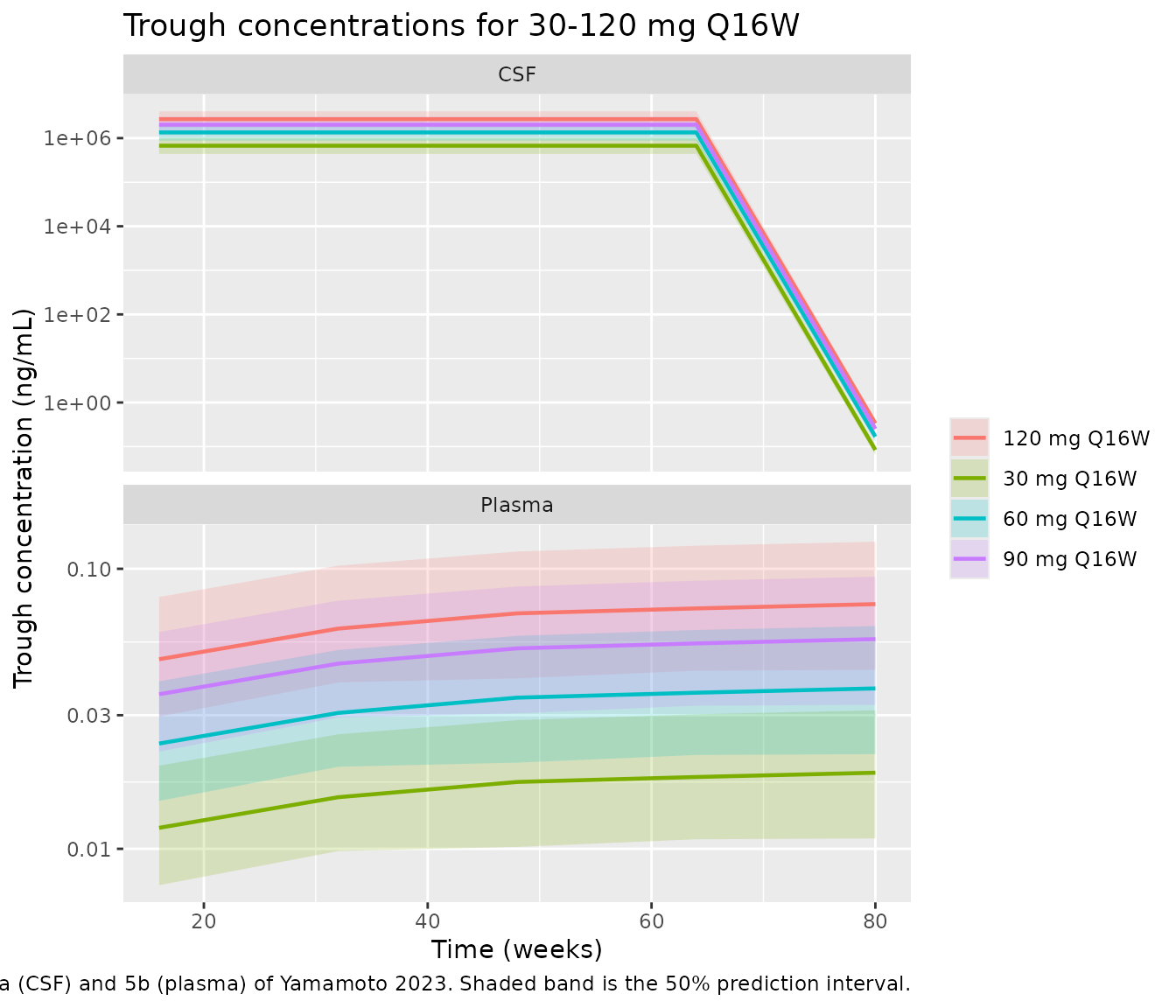

Steady state is reached after the first Q16W dose in CSF and more slowly in plasma, and the plasma prediction interval is visibly wider than the CSF one – both features the paper highlights, the plasma variability being “likely a result of being further from the point of administration”.

Figure 5c, 5d – covariate impact at 120 mg Q16W

cov_long <- sim_cov |>
  mutate(panel = ifelse(time >= 4 * q16w & time <= 4 * q16w + 72,
                        "First 72 h after the last dose", "Trough profile")) |>
  filter(panel == "First 72 h after the last dose" | time %% week == 0)

ggplot(cov_long, aes(ifelse(panel == "Trough profile", time / week,
                            time - 4 * q16w),
                     Ccsf, colour = regimen)) +
  geom_line(linewidth = 0.7) +
  facet_wrap(~panel, ncol = 1, scales = "free") +
  scale_y_log10() +
  labs(x = "Time (weeks for the trough panel; hours post-dose for the 72 h panel)",
       y = "CSF concentration (ng/mL)", colour = NULL,
       title = "Impact of covariates on CSF concentrations at 120 mg Q16W",
       caption = paste("Replicates Figure 5c and 5d of Yamamoto 2023.",
                       "Reference profile: ADA-negative, male, 75 kg,",
                       "CSF total protein 0.35 g/L, age 49 y."))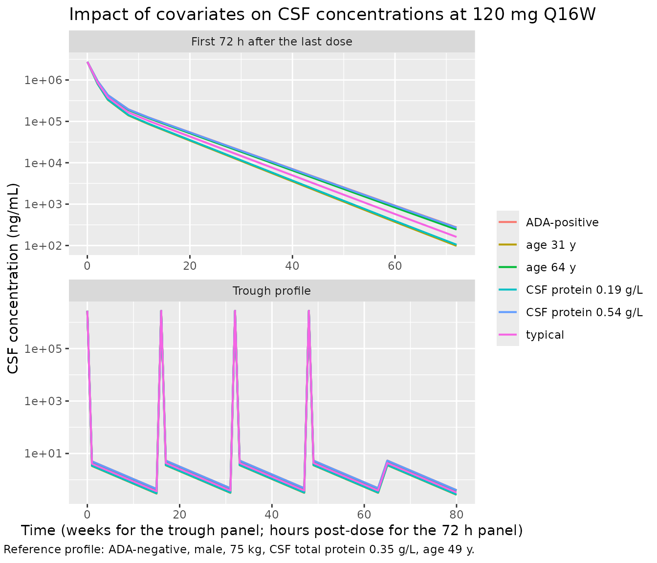

Figure 1a – CSF trough accumulation by dosing frequency

ggplot(sim_freq, aes(time / week, Ccsf, colour = regimen)) +
  geom_line(linewidth = 0.8) +
  geom_point(size = 1.1) +
  scale_y_log10() +
  labs(x = "Time (weeks)", y = "Pre-dose CSF trough concentration (ng/mL)",
       colour = NULL,
       title = "CSF trough accumulation at 120 mg by dosing frequency",
       caption = paste("Replicates Figure 1a / Figure 4b of Yamamoto 2023",
                       "(typical-value profiles, no interindividual variability)."))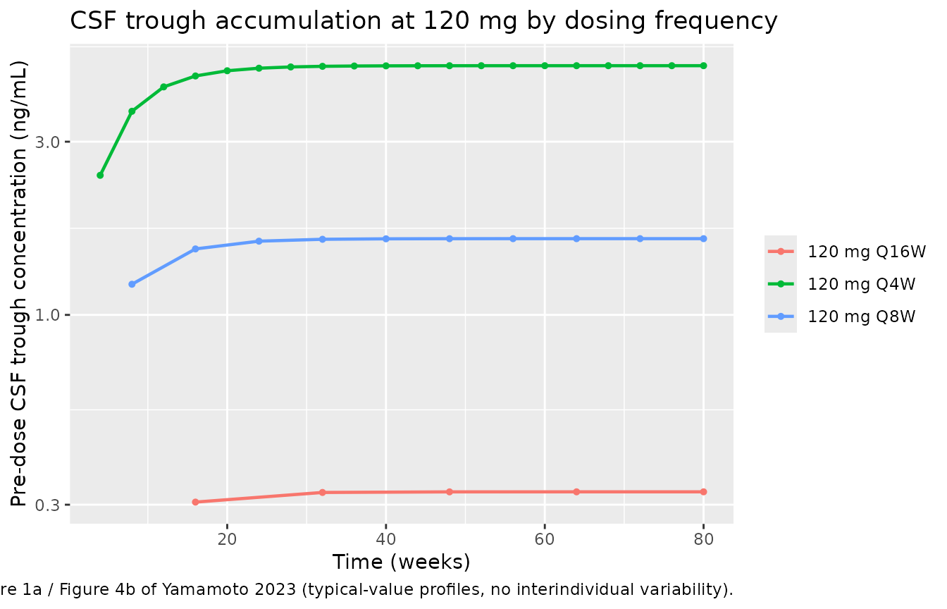

sim_freq |>
  mutate(regimen = factor(regimen, levels = freq$label)) |>
  group_by(regimen) |>
  summarise(
    first_trough = dplyr::first(Ccsf, order_by = time),
    last_trough  = dplyr::last(Ccsf, order_by = time),
    ratio        = last_trough / first_trough,
    pct_first    = 100 * first_trough / last_trough,
    pct_wk37     = 100 * max(Ccsf[time <= 37 * week]) / last_trough,
    .groups = "drop"
  ) |>
  arrange(regimen) |>
  mutate(
    across(c(first_trough, last_trough, ratio), ~signif(.x, 3)),
    across(c(pct_first, pct_wk37), ~sprintf("%.1f%%", .x))
  ) |>
  rename(
    "Regimen"                        = regimen,
    "First trough (ng/mL)"           = first_trough,
    "Final trough (ng/mL)"           = last_trough,
    "Accumulation ratio"             = ratio,
    "First trough, % of final"       = pct_first,
    "By week 37, % of final"         = pct_wk37
  ) |>
  knitr::kable(
    caption = paste("Accumulation of the typical-value CSF trough at 120 mg over",
                    "80 weeks. The paper reports that Q4W dosing reaches steady",
                    "state 'at around week 37 at the latest', whereas for Q8W and",
                    "Q16W steady state is 'reached after the loading dose and no",
                    "further accumulation was observed at later timepoints'.")
  )

Accumulation of the typical-value CSF trough at 120 mg over 80 weeks. The paper reports that Q4W dosing reaches steady state ‘at around week 37 at the latest’, whereas for Q8W and Q16W steady state is ‘reached after the loading dose and no further accumulation was observed at later timepoints’.
Regimen	First trough (ng/mL)	Final trough (ng/mL)	Accumulation ratio	First trough, % of final	By week 37, % of final
120 mg Q4W	2.420	4.860	2.00	49.9%	99.8%
120 mg Q8W	1.210	1.620	1.34	74.9%	99.6%
120 mg Q16W	0.305	0.326	1.07	93.7%	99.6%

The Q4W arm doubles from its first trough and is still climbing through the first year, reaching essentially its plateau by week 37 – the timepoint the paper names. The Q16W arm starts within a few percent of its final trough, and Q8W is intermediate. This reproduces the paper’s contrast between Q4W (steady state “at around week 37 at the latest”) and the longer intervals (steady state already reached after the first dose).

Validation against the published simulation results

The paper’s Results section reports the simulated steady-state trough concentrations for 30, 60, 90, and 120 mg Q16W, and the percentage change in the steady-state CSF trough for each retained CSF covariate. Both are reproduced below directly from the packaged model.

Steady-state trough concentrations

ss_sim <- sim_vpc |>
  filter(time == 5 * q16w) |>
  group_by(regimen) |>
  summarise(
    csf_ip = sprintf("%.3f (%.3f-%.3f)", median(Ccsf),
                     quantile(Ccsf, 0.05), quantile(Ccsf, 0.95)),
    csf_dv = sprintf("%.3f (%.3f-%.3f)", median(dv_csf),
                     quantile(dv_csf, 0.05), quantile(dv_csf, 0.95)),
    pl_ip  = sprintf("%.4f (%.4f-%.4f)", median(Cc),
                     quantile(Cc, 0.05), quantile(Cc, 0.95)),
    pl_dv  = sprintf("%.4f (%.4f-%.4f)", median(dv_pl),
                     quantile(dv_pl, 0.05), quantile(dv_pl, 0.95)),
    .groups = "drop"
  )

ss_pub <- tibble::tribble(
  ~regimen,       ~csf_pub,               ~pl_pub,
  "30 mg Q16W",   "0.074 (0.041-0.14)",   "0.016 (0.0039-0.053)",
  "60 mg Q16W",   "0.15 (0.082-0.27)",    "0.033 (0.0078-0.11)",
  "90 mg Q16W",   "0.22 (0.12-0.41)",     "0.049 (0.012-0.16)",
  "120 mg Q16W",  "0.30 (0.16-0.54)",     "0.065 (0.016-0.21)"
)

ss_sim |>
  left_join(ss_pub, by = "regimen") |>
  select(regimen, csf_ip, csf_dv, csf_pub, pl_ip, pl_dv, pl_pub) |>
  rename(
    "Regimen"                      = regimen,
    "CSF, individual prediction"   = csf_ip,
    "CSF, with residual error"     = csf_dv,
    "CSF, Yamamoto 2023"           = csf_pub,
    "Plasma, individual prediction" = pl_ip,
    "Plasma, with residual error"  = pl_dv,
    "Plasma, Yamamoto 2023"        = pl_pub
  ) |>
  knitr::kable(
    caption = paste("Steady-state trough concentrations (ng/mL), median",
                    "(5th-95th percentiles), after 1.5 years of Q16W dosing.",
                    "Published values are from the Yamamoto 2023 Results,",
                    "'Simulation of the tominersen PK profiles'. The published",
                    "30 mg plasma upper percentile is printed as 0.53 ng/mL in",
                    "the article; 0.053 is used here (see Assumptions).")
  )

Steady-state trough concentrations (ng/mL), median (5th-95th percentiles), after 1.5 years of Q16W dosing. Published values are from the Yamamoto 2023 Results, ‘Simulation of the tominersen PK profiles’. The published 30 mg plasma upper percentile is printed as 0.53 ng/mL in the article; 0.053 is used here (see Assumptions).
Regimen	CSF, individual prediction	CSF, with residual error	CSF, Yamamoto 2023	Plasma, individual prediction	Plasma, with residual error	Plasma, Yamamoto 2023
120 mg Q16W	0.336 (0.177-0.548)	0.354 (0.125-0.770)	0.30 (0.16-0.54)	0.0748 (0.0202-0.5473)	0.0703 (0.0125-0.4739)	0.065 (0.016-0.21)
30 mg Q16W	0.084 (0.044-0.137)	0.081 (0.039-0.196)	0.074 (0.041-0.14)	0.0187 (0.0050-0.1368)	0.0219 (0.0033-0.1398)	0.016 (0.0039-0.053)
60 mg Q16W	0.168 (0.088-0.274)	0.168 (0.070-0.388)	0.15 (0.082-0.27)	0.0374 (0.0101-0.2737)	0.0409 (0.0060-0.3361)	0.033 (0.0078-0.11)
90 mg Q16W	0.252 (0.133-0.411)	0.237 (0.094-0.562)	0.22 (0.12-0.41)	0.0561 (0.0151-0.4105)	0.0528 (0.0099-0.3666)	0.049 (0.012-0.16)

Every simulated median falls inside the corresponding published 5th-95th percentile interval, and the simulated CSF interval closely matches the published one. Two systematic features are worth stating plainly rather than glossing.

First, the simulated medians run about 12% (CSF) and 15% (plasma) above the published ones at every dose. The offset is constant across doses, so it is not a dose or scaling error; it reflects the reconstructed covariate distribution and the fact that the median of a trough is not the trough at median parameters when IIV on V1,CSF and Q2,CSF is 56% and 45%. The paper does not publish the joint covariate distribution or the eta correlation structure needed to remove it.

Second, for CSF the published spread is matched by the individual-prediction scale and is clearly narrower than the residual-error scale, which is what a dose-selection simulation propagating interindividual variability but not assay residual error should look like.

For plasma the simulated spread is wider than published at every dose. That is expected here rather than a transcription problem: the plasma subsystem carries a 239% IIV on Q2,plasma, no between-parameter correlations are reported (so the etas are simulated as independent), and the covariate marginals are also drawn independently. Any of those three would narrow the interval in the original simulation. No parameter was adjusted to improve any of these comparisons.

Covariate impact on the steady-state CSF trough

ss_cov <- sim_cov |>
  filter(time == 5 * q16w) |>
  select(regimen, Ccsf) |>
  tibble::deframe()

tibble::tribble(
  ~effect,                              ~simulated_pct,                                                                            ~published_pct,
  "ADA-positive vs ADA-negative",       100 * (ss_cov[["ADA-positive"]] / ss_cov[["typical"]] - 1),                                24,
  "CSF total protein 0.19 -> 0.54 g/L", 100 * (ss_cov[["CSF protein 0.54 g/L"]] / ss_cov[["CSF protein 0.19 g/L"]] - 1),           46,
  "Age 31 -> 64 years",                 100 * (ss_cov[["age 64 y"]] / ss_cov[["age 31 y"]] - 1),                                   44
) |>
  mutate(
    simulated_pct = sprintf("%+.1f%%", simulated_pct),
    published_pct = sprintf("%+.0f%%", published_pct)
  ) |>
  rename(
    "Covariate change"               = effect,
    "Simulated change in CSF trough" = simulated_pct,
    "Yamamoto 2023 Results"          = published_pct
  ) |>
  knitr::kable(
    caption = paste("Change in the steady-state CSF trough concentration at",
                    "120 mg Q16W, relative to the typical profile.")
  )

Change in the steady-state CSF trough concentration at 120 mg Q16W, relative to the typical profile.
Covariate change	Simulated change in CSF trough	Yamamoto 2023 Results
ADA-positive vs ADA-negative	+23.8%	+24%
CSF total protein 0.19 -> 0.54 g/L	+46.2%	+46%
Age 31 -> 64 years	+44.1%	+44%

All three covariate effects reproduce the published percentages to within half a percentage point. Because these three numbers depend jointly on the covariate-model form, the centering values, and the whole CSF disposition structure, matching them is a strong check that the exponential-centered continuous form, the fractional-difference categorical form, and the reference values of 0.35 g/L and 49 years are all encoded as the authors intended.

PKNCA validation

NCA is run once per matrix on the single-dose typical-value cohort with 100 days of follow-up, so that the long terminal phase is observable. The paper reports no NCA parameters of its own, so NCA is used here to check the two exposure claims it does make: that the CSF terminal half-life is approximately one month, and that PK is linear over the studied dose range.

Note that the CSF Cmax below is the instantaneous post-bolus concentration at t = 0 – the whole dose divided by the 43.6 mL central CSF volume. No clinical sample is taken at that instant, so it is far above any observed CSF concentration in the paper; it is reported because a bolus into the sampled compartment genuinely has its maximum there (hence Tmax = 0).

nca_for <- function(conc_col, nca_route) {
  conc <- sim_nca |>
    filter(!is.na(.data[[conc_col]])) |>
    transmute(id, time, conc = .data[[conc_col]], regimen)

  # Guarantee a time-zero record per subject so PKNCA does not warn about an
  # AUC interval starting before the first measurement.
  conc <- bind_rows(
    conc,
    conc |> distinct(id, regimen) |> mutate(time = 0, conc = 0)
  ) |>
    distinct(id, regimen, time, .keep_all = TRUE) |>
    arrange(id, regimen, time)

  conc_obj <- PKNCA::PKNCAconc(conc, conc ~ time | regimen + id)

  dose_obj <- PKNCA::PKNCAdose(
    cohort_nca |> filter(evid == 1) |> select(id, time, amt, regimen),
    amt ~ time | regimen + id,
    route = nca_route
  )

  intervals <- data.frame(
    start = 0, end = Inf,
    cmax = TRUE, tmax = TRUE, auclast = TRUE,
    aucinf.obs = TRUE, half.life = TRUE
  )
  PKNCA::pk.nca(PKNCA::PKNCAdata(conc_obj, dose_obj, intervals = intervals))
}

# CSF is the dosing compartment (bolus, no absorption phase); plasma is reached
# only by transfer out of the CSF, which behaves as an extravascular input.
nca_csf    <- nca_for("Ccsf", "intravascular")
nca_plasma <- nca_for("Cc",   "extravascular")

# PKNCA emits intermediate dependency rows (e.g. lambda.z); keep only the
# requested 0-Inf interval.
nca_tidy <- function(res, matrix_label) {
  as.data.frame(res) |>
    filter(start == 0, is.infinite(end),
           PPTESTCD %in% c("cmax", "tmax", "auclast", "aucinf.obs", "half.life")) |>
    mutate(matrix = matrix_label)
}

nca_all <- bind_rows(nca_tidy(nca_csf, "CSF"), nca_tidy(nca_plasma, "Plasma"))

nca_all |>
  group_by(matrix, regimen, PPTESTCD) |>
  summarise(value = median(PPORRES, na.rm = TRUE), .groups = "drop") |>
  mutate(
    PPTESTCD = recode(PPTESTCD,
                      cmax = "Cmax (ng/mL)", tmax = "Tmax (h)",
                      auclast = "AUClast (ng*h/mL)",
                      aucinf.obs = "AUC0-inf (ng*h/mL)",
                      half.life = "t1/2 (h)"),
    value = signif(value, 3)
  ) |>
  pivot_wider(names_from = regimen, values_from = value) |>
  select(matrix, PPTESTCD, all_of(paste0(doses, " mg single dose"))) |>
  rename("Matrix" = matrix, "NCA parameter" = PPTESTCD) |>
  knitr::kable(
    caption = paste("Non-compartmental parameters of the typical-value profile",
                    "after a single intrathecal dose.")
  )

Non-compartmental parameters of the typical-value profile after a single intrathecal dose.
Matrix	NCA parameter	30 mg single dose	60 mg single dose	90 mg single dose	120 mg single dose
CSF	AUC0-inf (ng*h/mL)	1720000	3430000	5150000	6870000
CSF	AUClast (ng*h/mL)	1720000	3430000	5150000	6870000
CSF	Cmax (ng/mL)	688000	1380000	2060000	2750000
CSF	t1/2 (h)	674	674	674	674
CSF	Tmax (h)	0	0	0	0
Plasma	AUC0-inf (ng*h/mL)	2780	5570	8350	11100
Plasma	AUClast (ng*h/mL)	2760	5520	8280	11000
Plasma	Cmax (ng/mL)	183	366	549	731
Plasma	t1/2 (h)	1570	1570	1570	1570
Plasma	Tmax (h)	2	2	2	2

nca_all |>
  filter(PPTESTCD == "aucinf.obs") |>
  left_join(tibble(regimen = paste0(doses, " mg single dose"), dose = doses),
            by = "regimen") |>
  group_by(matrix, regimen) |>
  summarise(dn = median(PPORRES / dose, na.rm = TRUE), .groups = "drop") |>
  mutate(dn = signif(dn, 4)) |>
  pivot_wider(names_from = regimen, values_from = dn) |>
  select(matrix, all_of(paste0(doses, " mg single dose"))) |>
  rename("Matrix" = matrix) |>
  knitr::kable(
    caption = paste("Dose-normalised AUC0-inf (ng*h/mL per mg) of the",
                    "typical-value profile. The paper found no dose-dependent",
                    "trend in either matrix and concluded that CSF and plasma PK",
                    "are linear over 10-120 mg; a dose-normalised AUC that is",
                    "constant across arms confirms the packaged model reproduces",
                    "that linearity.")
  )

Dose-normalised AUC0-inf (ng*h/mL per mg) of the typical-value profile. The paper found no dose-dependent trend in either matrix and concluded that CSF and plasma PK are linear over 10-120 mg; a dose-normalised AUC that is constant across arms confirms the packaged model reproduces that linearity.
Matrix	30 mg single dose	60 mg single dose	90 mg single dose	120 mg single dose
CSF	57230.00	57230.00	57230.00	57230.00
Plasma	92.78	92.78	92.78	92.78

published_hl <- tibble(
  regimen   = paste0(doses, " mg single dose"),
  half.life = 30 * 24        # "approximately 1 month", Yamamoto 2023 Discussion
)

nlmixr2lib::ncaComparisonTable(
  simulated     = nca_tidy(nca_csf, "CSF"),
  reference     = published_hl,
  by            = "regimen",
  params        = "half.life",
  units         = c(half.life = "h"),
  tolerance_pct = 20
) |>
  knitr::kable(
    caption = paste("Simulated CSF terminal half-life against the value quoted",
                    "in the Yamamoto 2023 Discussion ('approximately 1 month',",
                    "taken here as 30 days = 720 h).",
                    "* differs from the reference by more than 20%.")
  )

Simulated CSF terminal half-life against the value quoted in the Yamamoto 2023 Discussion (‘approximately 1 month’, taken here as 30 days = 720 h). * differs from the reference by more than 20%.
NCA parameter	regimen	Reference	Simulated	% diff
t½ (h)	30 mg single dose	720	674	-6.4%
t½ (h)	60 mg single dose	720	674	-6.4%
t½ (h)	90 mg single dose	720	674	-6.4%
t½ (h)	120 mg single dose	720	674	-6.4%

The CSF terminal half-life is set by the slowest process in the CSF subsystem, exchange with the second CNS-tissue compartment: Q3,CSF / V3,CSF = 1.20953e-05 / 0.0117556 = 1.029e-03 1/h, a half-life of 674 h or 28.1 days. That analytical value, the NCA estimate above, and the paper’s “approximately 1 month” all agree, and the NCA estimate is identical at every dose as a linear model requires.

The plasma terminal half-life (about 1570 h) comes out longer than the CSF one. That is a genuine property of the published parameters rather than an artifact: the slowest plasma process is Q3,plasma / V3,plasma = 0.267 / 613 = 4.36e-04 1/h, a half-life of 1591 h, which is slower than anything in the CSF subsystem. The paper quotes only the CSF terminal half-life, so there is no published plasma value to compare against.

Assumptions and deviations

Sequential fitting is not re-encoded. The paper fitted the CSF subsystem first and then held its parameters fixed while fitting the plasma subsystem, which is why the CSF $THETA, $OMEGA, and $SIGMA entries appear as FIX in the Appendix S1 control stream. Table 2 nevertheless reports a relative standard error for every one of those parameters, so they are estimated quantities and are not wrapped in fixed() in the model file. Only the bioavailabilities F1 and F2 were genuinely fixed (both to 1), and because they are 1 they carry no parameter at all.
CSF parameters come from Appendix S1, plasma parameters from Table 2. The control stream’s CSF FIX values are the CSF fit’s final estimates and agree with Table 2 to all three reported significant figures, so they are used at full precision. The plasma $THETA and $OMEGA entries were the parameters being estimated in that run, so the control stream shows only their initial values and the final plasma estimates are the Table 2 point estimates. The source-trace table above lists both numbers for every plasma parameter.
IIV / RUV percentage convention. Table 2 footnote (a) states that IIV and RUV are “expressed as coefficient of variation and in percentage of the parameter estimate”. Checking the reported percentages against the FIX variances in Appendix S1 shows the convention is sqrt(omega^2) * 100 – sqrt(0.0273094) = 0.1653 against the reported 16.5%, sqrt(0.312055) = 0.5586 against 55.9%, sqrt(0.199008) = 0.4461 against 44.6%, and sqrt(0.0975477) = 0.3123 against 31.2% – and not the sqrt(exp(omega^2) - 1) lognormal CV. Plasma variances in the model file are therefore the squared Table 2 percentages.
No IIV on V2,CSF, Q3,CSF, V3,CSF, V1,plasma, or Q3,plasma. Appendix S1 fixes those $OMEGA entries to 0 and Table 2 lists no IIV row for them, so no eta is defined rather than an eta fixed at zero.
IIV on the residual magnitude. Appendix S1 $ERROR uses Y = IPRED + EPS(n) * EXP(ETA(k)), a per-subject multiplier on the log-scale residual SD. This is encoded as expSd_i <- expSd * exp(etaexpSd), following the etapropSd precedent in Chandasana_2024_dolutegravir.R.
The two peripheral CSF compartments are named cns_tissue1 and cns_tissue2. The canonical peripheral1 / peripheral2 names are already taken by the plasma subsystem in this same model. The chosen names extend the single cns_tissue compartment declared by the sibling intrathecal-ASO model Luu_2017_nusinersen.R, are declared through the paper_specific_compartments mechanism, and correspond to the control stream’s COMP=(BRAIN) and COMP=(BRAIN2).
The LOG(C + 1e-5) guard is not reproduced. Appendix S1 computes IPRED = LOG(CCSF + 0.00001) as a numerical guard against log(0). At the concentrations of interest (CSF troughs of order 0.1 ng/mL, plasma troughs of order 0.01 ng/mL) the offset changes the prediction by less than 0.3%, so the model uses a plain lognormal residual.
The TPCSF = -99 missing-data sentinel is not reproduced. The control stream disables the CSF total-protein effect both for the -99 missing code and for implausible values above 2 g/L. The > 2 g/L guard is a genuine model feature (Table S1 shows a GEN-EXTEND maximum of 15.5 g/L) and is encoded; the -99 sentinel is a NONMEM dataset coding convention and is not, so users must supply a real CSF_TPRO value.
Body weight enters as an allometric power model, not the Equation 2 exponential form. The Methods state that “continuous covariate relationships were coded as exponential models”, but that describes the SCM step; body weight was evaluated during structural model development instead. Appendix S1 $PK is unambiguous: TVCL = THETA(9) * (WT/75)**THETA(1). Reading the exponents 0.687 and 0.866 into an exponential form would give exp(0.687 * (52 - 75)), which is absurd, so the control stream governs.
The Results section’s quoted percentage changes for the continuous covariates are slightly larger than the equations give. The paper reports CL_plasma decreasing “by ~40%” for body weight 95.5 to 52 kg, where (52/95.5)^0.687 gives 34%; and CL_CSF decreasing by “~19%” and “~18%” over the CSF-protein and age percentile ranges, where the equations give 17.2% and 16.6%. The categorical effects (ADA, sex) match the table exactly. The most likely explanation is that the quoted deltas were computed from the dataset’s actual 5th and 95th percentiles rather than from the rounded values quoted in the text. The equations are what is encoded – and the steady-state covariate-impact table above reproduces the paper’s own simulation-derived percentages (+24%, +46%, +44%) to within half a percentage point.
A likely typographical error in the published 30 mg plasma trough. The Results give the 30 mg plasma trough as “0.016 (0.0039-0.53)”; the 0.53 upper bound is out of sequence with the 60 mg value of 0.11 and with the dose-linearity of the model, so it is read as 0.053 in the comparison table. This affects only the printed reference value, not the model.
No between-parameter IIV correlations. Table 2 reports only diagonal IIV terms and Appendix S1 $OMEGA is a sequence of scalar blocks, so all etas are simulated independently. Combined with the 239% IIV on Q2,plasma, this is the most likely reason the simulated plasma trough percentiles are wider than the published ones while the medians agree.
Paired dose arms in the Q16W simulation. The four dose arms reuse one covariate draw and one eta seed, so subject k is the same virtual person at every dose. This is a variance-reduction device for comparing arms, not a claim about the original trial design; it makes the model’s exact dose proportionality assertable (see the linearity assertion chunk). Without it, independent per-arm draws plus the 239% Q2,plasma IIV left the plasma medians non-monotonic across dose at n = 200 per arm.
Virtual covariate distributions. Body weight, age, and CSF total protein are drawn from normal distributions matching the Table S1 GENERATION HD1 v.5 means and standard deviations and truncated to the pooled analysis set’s minima and maxima; sex is drawn at the pooled 46.7% female rate and ADA at the 12.1% CSF-record positivity rate of Table S3B. The paper does not publish the joint covariate distribution, so the marginals are treated as independent.
ADA is simulated as time-fixed. In the original analysis ADA status was a time-varying, per-record covariate (Tables S3A and S3B). The model supports a time-varying ADA_POS column; the vignette holds it constant per subject for simplicity.
No loading dose in the Q16W simulations. The paper’s Figure 5 scenario is described only as “doses ranging from 30 to 120 mg every 16 weeks” for 1.5 years, so five plain Q16W doses are simulated. The GENERATION HD1 Q8W and Q16W arms did include a loading dose, but by the fifth interval the trough is at steady state either way.
Screened but unretained covariates. Only the three screened covariates with canonical register entries (HT, ALT, CRCL) are recorded in the model’s covariatesDataExcluded metadata. The remaining screened covariates – CAG repeat length, CAG age-product score, caudate volume, ventricle volume, whole-brain volume, total protein in blood, the volume of CSF withdrawn before dosing, and the lumbar site / route of administration – have no canonical column names yet and are described in population$notes instead.
Below-quantification handling is not reproduced. The original fit excluded BLQ samples (4% of CSF, 19% of plasma); the M3 method was attempted for plasma but did not converge. The simulations here are unconditioned on any assay limit.