Iptacopan plasma binding to factor B in hepatic impairment (Burmeister Getz 2025)
Source:vignettes/articles/BurmeisterGetz_2025_iptacopan.Rmd
BurmeisterGetz_2025_iptacopan.RmdModel and source
- Citation: Burmeister Getz E, Stein RR, Fink M, Kulmatycki K, Baltcheva I, Weis W, Shah B, Lawitz E, Schmouder R. Effect of Target-Mediated Disposition on Iptacopan Clinical Pharmacokinetics in Participants with Normal or Impaired Hepatic Function. Clin Pharmacol Ther. 2025;117(5):1358-1368. doi:10.1002/cpt.3559.
- Article: Clin Pharmacol Ther 2025;117(5):1358-1368 (open access; PMC11993288). The Supplementary Appendix (Data S1) holds the derivation of the binding model.
Iptacopan is an oral inhibitor of complement factor B, a soluble, hepatically produced plasma protein (about 150 ug/mL) that iptacopan binds with nanomolar affinity. Because factor B is abundant but saturable at the clinical dose, iptacopan shows small-molecule target-mediated drug disposition: its unbound fraction falls as total concentration falls. In the phase I hepatic-impairment study CLNP023A2105 every plasma sample was assayed for both total and unbound iptacopan, and Burmeister Getz et al. fitted a two-site competitive equilibrium binding model to the paired concentrations:
(unbound drug, drug bound to factor B, drug bound non-specifically to the other plasma proteins; Figure 2a). The model has no time dependence. The packaged form takes total iptacopan as a time-varying covariate and returns the unbound concentration from the single meaningful root of that quadratic (main-text equation; Supplementary Appendix eq. 2),
together with the fractional occupancy of available factor B,
occ = Cu / (KD + Cu) (Supplementary Appendix eq. 3).
The authors fitted the model separately to each hepatic-function group, so the library carries four models with the same structure and group-specific parameters:
models <- c(
  "Healthy controls" = "BurmeisterGetz_2025_iptacopan_healthy",
  "Mild HI" = "BurmeisterGetz_2025_iptacopan_mild_hepatic",
  "Moderate HI" = "BurmeisterGetz_2025_iptacopan_moderate_hepatic",
  "Severe HI" = "BurmeisterGetz_2025_iptacopan_severe_hepatic"
)
group_levels <- names(models)
mw_iptacopan <- 422.52 # g/mol, Table 3 footnote b

pars <- lapply(models, function(m) {
  th <- rxode2::rxode(readModelDb(m))$theta
  c(bmax = exp(th[["lbmax"]]), kd = exp(th[["lkd"]]), fumax = th[["fumax"]])
})
par_tab <- dplyr::bind_rows(lapply(pars, as.list), .id = "group")
knitr::kable(par_tab, digits = c(0, 2, 2, 2))| group | bmax | kd | fumax |
|---|---|---|---|
| Healthy controls | 1874.30 | 9.63 | 0.25 |
| Mild HI | 1775.56 | 10.89 | 0.32 |
| Moderate HI | 1403.16 | 8.00 | 0.34 |
| Severe HI | 880.36 | 8.84 | 0.49 |
Population
38 adults received a single fasted oral 200 mg dose of iptacopan at a single site: 16 healthy controls, 8 with mild (Child-Pugh A, score 5-6), 8 with moderate (Child-Pugh B, 7-9) and 6 with severe (Child-Pugh C, 10-15) hepatic impairment (HI). Each HI participant was matched to a healthy control by sex, age (+/- 10 years), body weight (+/- 15%) and smoking status. Median age was 59.5 years (31-75), median weight 86.8 kg (59.5-116.0), 47.4% were female and 94.7% White (Table 1). Serum albumin fell from a median 44.5 g/L in controls to 30.5 g/L in severe HI, and bilirubin rose from 6.8 to 50.5 umol/L. Total and unbound iptacopan were measured at 22 post-dose times from 15 min to 240 h.
Each model’s population metadata carries its own group’s
demographics:
pop_tab <- dplyr::bind_rows(lapply(models, function(m) {
  p <- rxode2::rxode(readModelDb(m))$population
  data.frame(
    N = p$n_subjects,
    `Age, median (range)` = paste0(p$age_median, " (", p$age_range, ")"),
    `Weight range` = p$weight_range,
    `Female (%)` = p$sex_female_pct,
    check.names = FALSE
  )
}), .id = "Group")
knitr::kable(pop_tab)| Group | N | Age, median (range) | Weight range | Female (%) |
|---|---|---|---|---|
| Healthy controls | 16 | 60.5 years (31-73 years) | 59.5-112.6 kg | 43.8 |
| Mild HI | 8 | 63.5 years (50-75 years) | 72.1-116.0 kg | 37.5 |
| Moderate HI | 8 | 61.5 years (53-70 years) | 65.5-112.8 kg | 50.0 |
| Severe HI | 6 | 54.0 years (31-60 years) | 66.9-101.9 kg | 66.7 |
Source trace
The per-parameter origin is recorded as an in-file comment next to
each ini() entry in
inst/modeldb/specificDrugs/BurmeisterGetz_2025_iptacopan_*.R.
| Equation / parameter | Healthy | Mild HI | Moderate HI | Severe HI | Source location |
|---|---|---|---|---|---|
lbmax (fB,avail, nM) |
log(1874.30) | log(1775.56) | log(1403.16) | log(880.36) | Table 3, row ‘fB,avail, nM (ug/mL)’ |
lkd (KD, nM) |
log(9.63) | log(10.89) | log(8.00) | log(8.84) | Table 3, row ‘KD, nM’ |
fumax |
0.25 | 0.32 | 0.34 | 0.49 | Table 3, row ‘fu,max’ |
propSd |
fixed(0) | fixed(0) | fixed(0) | fixed(0) | Supplementary Appendix ‘Statistical analyses’ (proportional error; magnitude not reported) |
| Molecular weight 422.52 g/mol | Table 3 footnote b | ||||
| Binding equation (total from unbound) | Figure 2a; Supplementary Appendix eq. 1 | ||||
| Closed-form unbound concentration | Main-text equation after Figure 3; Supplementary Appendix eq. 2 | ||||
Factor B occupancy Cu / (KD + Cu)
|
Main text ‘Target occupancy throughout the dosing interval’; Supplementary Appendix eq. 3 |
Simulation
Because the model is algebraic, a “simulation” evaluates it on a grid
of total concentrations. Each grid point is an observation record;
time is a dummy index.
ctot_grid <- exp(seq(log(5), log(2e4), length.out = 200))

solve_group <- function(model_name, ctot) {
  ev <- data.frame(
    id = 1L,
    time = seq_along(ctot) - 1,
    evid = 0L,
    amt = 0,
    CP_IPTACOPAN_NGML = ctot
  )
  rxode2::rxSolve(readModelDb(model_name), events = ev, keep = "CP_IPTACOPAN_NGML") |>
    as.data.frame()
}

sim <- dplyr::bind_rows(
  lapply(models, solve_group, ctot = ctot_grid),
  .id = "group"
) |>
  dplyr::mutate(
    group = factor(group, levels = group_levels),
    ctot_nm = CP_IPTACOPAN_NGML * 1000 / mw_iptacopan,
    cu_nm = Cu * 1000 / mw_iptacopan
  )
Replicate published figures
Figure 2b – binding components in healthy controls
Total iptacopan against unbound iptacopan (both nM) for the healthy-control parameters, split into the three binding states of Figure 2a.
p_h <- pars[["Healthy controls"]]
fig2 <- sim |>
  dplyr::filter(group == "Healthy controls") |>
  dplyr::transmute(
    cu_nm,
    `Total` = ctot_nm,
    `Bound to factor B` = p_h[["bmax"]] * occ,
    `Unbound + non-specifically bound` = cu_nm / p_h[["fumax"]]
  ) |>
  tidyr::pivot_longer(-cu_nm, names_to = "component", values_to = "conc_nm")

ggplot(fig2, aes(cu_nm, conc_nm, colour = component, linetype = component)) +
  geom_line(linewidth = 0.8) +
  scale_x_log10() +
  scale_y_log10() +
  coord_cartesian(xlim = c(0.1, 1e4), ylim = c(10, 5e4)) +
  labs(
    x = "Unbound iptacopan (nM)",
    y = "Iptacopan (nM)",
    colour = NULL,
    linetype = NULL,
    caption = "Replicates Figure 2b of Burmeister Getz 2025 (model curves only)."
  ) +
  theme_bw() +
  theme(legend.position = "bottom")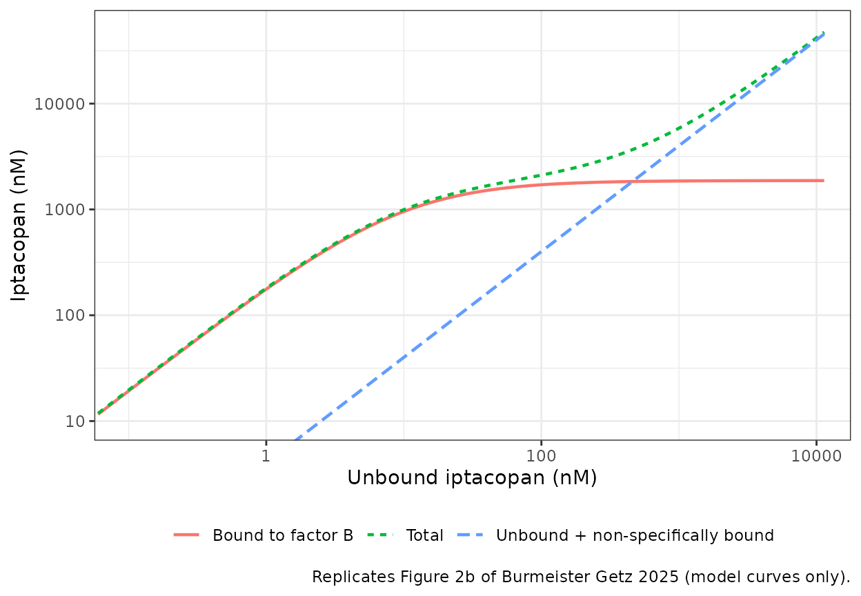
The factor B curve plateaus at fB,avail (1874 nM, about 790 ng/mL of iptacopan-equivalent) while the non-specific line rises with slope 1 / fu,max = 4, reproducing the shape of Figure 2b.
Figure 3a – multiphasic plasma protein binding by HI group
ggplot(sim |> dplyr::filter(Cu > 0.1), aes(Cu, CP_IPTACOPAN_NGML, colour = group)) +
  geom_line(linewidth = 0.8) +
  scale_x_log10() +
  scale_y_log10() +
  coord_cartesian(xlim = c(0.1, 2000), ylim = c(10, 1e4)) +
  labs(
    x = "Unbound iptacopan (ng/mL)",
    y = "Total iptacopan (ng/mL)",
    colour = NULL,
    caption = "Replicates Figure 3a of Burmeister Getz 2025 (model curves only)."
  ) +
  theme_bw()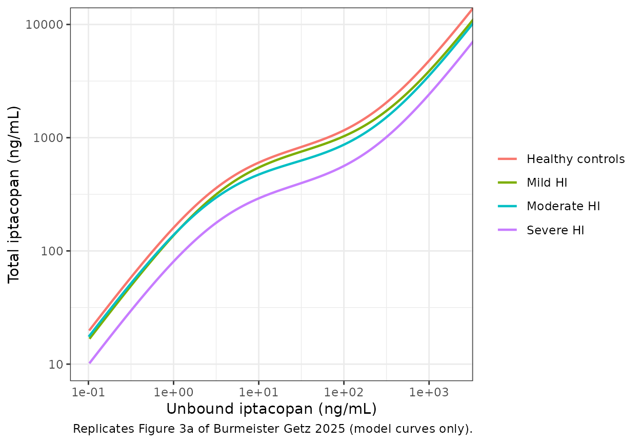
Figure 3b – factor B occupancy against total iptacopan
ec90_tab <- data.frame(
  group = factor(group_levels, levels = group_levels),
  ec90 = c(857.43, 804.09, 622.24, 403.04) # Table 3
)
ggplot(sim, aes(CP_IPTACOPAN_NGML, 100 * occ, colour = group)) +
  geom_line(linewidth = 0.8) +
  geom_vline(data = ec90_tab, aes(xintercept = ec90, colour = group), linetype = "dashed") +
  geom_hline(yintercept = 90, linetype = "dashed", colour = "grey40") +
  scale_x_log10() +
  coord_cartesian(xlim = c(10, 1e4)) +
  labs(
    x = "Total iptacopan (ng/mL)",
    y = "Estimated occupancy of available fB (%)",
    colour = NULL,
    caption = "Replicates Figure 3b of Burmeister Getz 2025; dashed verticals are the Table 3 EC90 values."
  ) +
  theme_bw()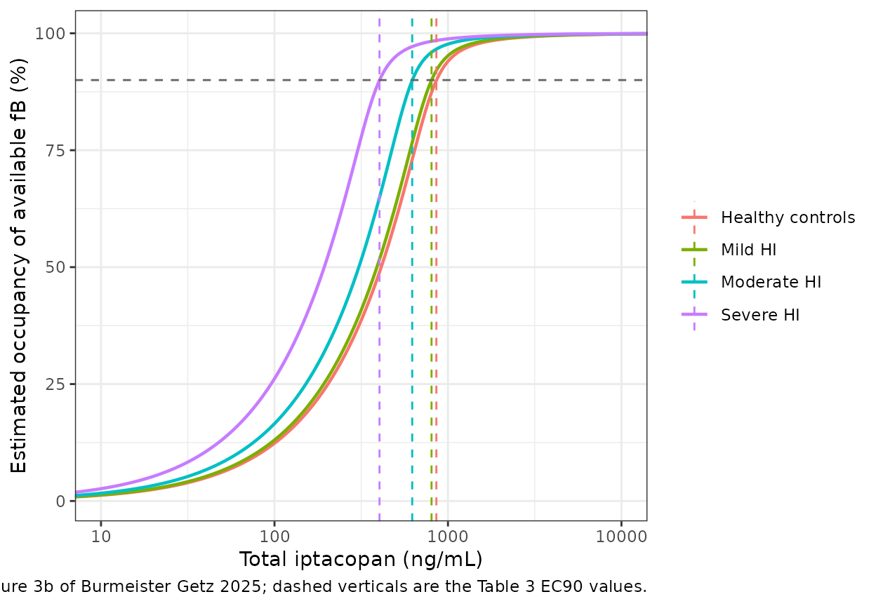
Figure 4 – unbound iptacopan and factor B activity over a dosing profile
Figure 4 transforms the mean total-iptacopan profile of the healthy controls (single 200 mg dose) into an unbound profile and a fractional factor B activity (100% minus occupancy). The three curves were digitised by the maintainers from the published figure at the times where each curve is legible (the peak region is hidden by the legend). The total-iptacopan readings drive the model; the unbound and activity readings are the targets.
fig4 <- data.frame(
  time = c(6, 8, 10, 12, 16, 20, 24, 36, 42, 48, 54, 60, 66, 72, 78, 84, 90),
  total = c(1773, 1425, 1178, 973, 849, 761, 670, 462, 418, 371, 296, 229, 181, 146, 115, 90.8, 72.3),
  unbound = c(253, 162, 90.8, NA, NA, 23.2, 14.0, NA, NA, 3.38, NA, NA, 1.20, 0.88, 0.70, 0.51, NA),
  activity = c(NA, 2.9, 4.8, 7.1, 12.1, 17.1, 22.3, 44.0, 49.8, 54.8, 61.8, 68.5, 75.7, 82.3, 85.1, 87.6, 90.5)
)

ev4 <- data.frame(
  id = 1L,
  time = fig4$time,
  evid = 0L,
  amt = 0,
  CP_IPTACOPAN_NGML = fig4$total
)
sim4 <- rxode2::rxSolve(
  readModelDb("BurmeisterGetz_2025_iptacopan_healthy"),
  events = ev4,
  keep = "CP_IPTACOPAN_NGML"
) |>
  as.data.frame()

fig4 <- fig4 |>
  dplyr::mutate(
    unbound_model = sim4$Cu,
    activity_model = 100 * (1 - sim4$occ),
    unbound_pct_diff = 100 * (unbound_model / unbound - 1),
    activity_diff = activity_model - activity
  )
fig4_long <- dplyr::bind_rows(
  data.frame(time = fig4$time, value = fig4$total, series = "Total (digitised, model input)", source = "Published"),
  data.frame(time = fig4$time, value = fig4$unbound, series = "Unbound", source = "Published"),
  data.frame(time = fig4$time, value = fig4$unbound_model, series = "Unbound", source = "Model")
) |>
  dplyr::filter(!is.na(value))

ggplot(fig4_long, aes(time, value, colour = series, shape = source, linetype = source)) +
  geom_point(size = 2) +
  geom_line() +
  scale_y_log10() +
  labs(
    x = "Nominal time after dosing (h)",
    y = "Mean iptacopan (ng/mL)",
    colour = NULL,
    shape = NULL,
    linetype = NULL,
    caption = "Replicates the concentration curves of Figure 4 of Burmeister Getz 2025."
  ) +
  theme_bw()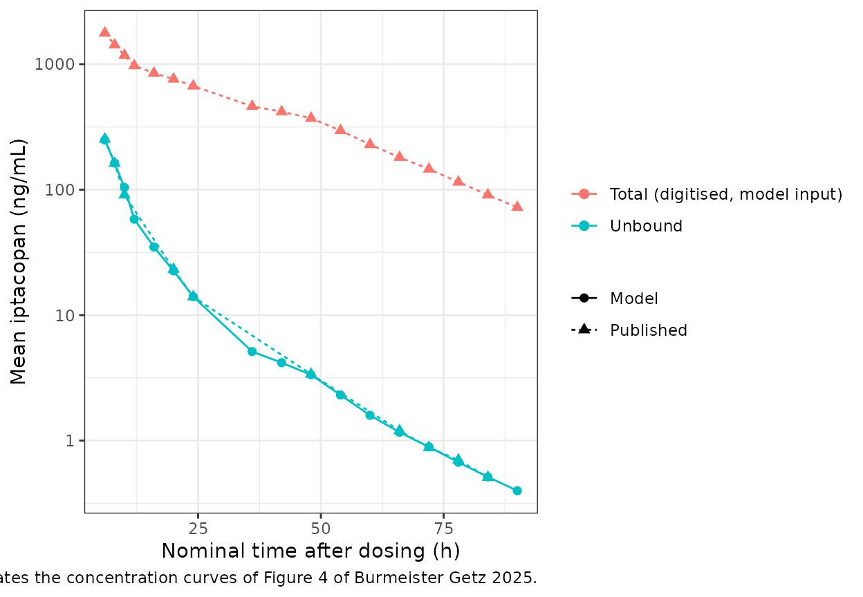
ggplot(fig4 |> dplyr::filter(!is.na(activity)), aes(time)) +
  geom_point(aes(y = activity, shape = "Published (digitised)"), size = 2) +
  geom_line(aes(y = activity_model, linetype = "Model")) +
  labs(
    x = "Nominal time after dosing (h)",
    y = "Fractional factor B activity (%)",
    shape = NULL,
    linetype = NULL,
    caption = "Replicates the factor B activity curve of Figure 4 of Burmeister Getz 2025."
  ) +
  theme_bw()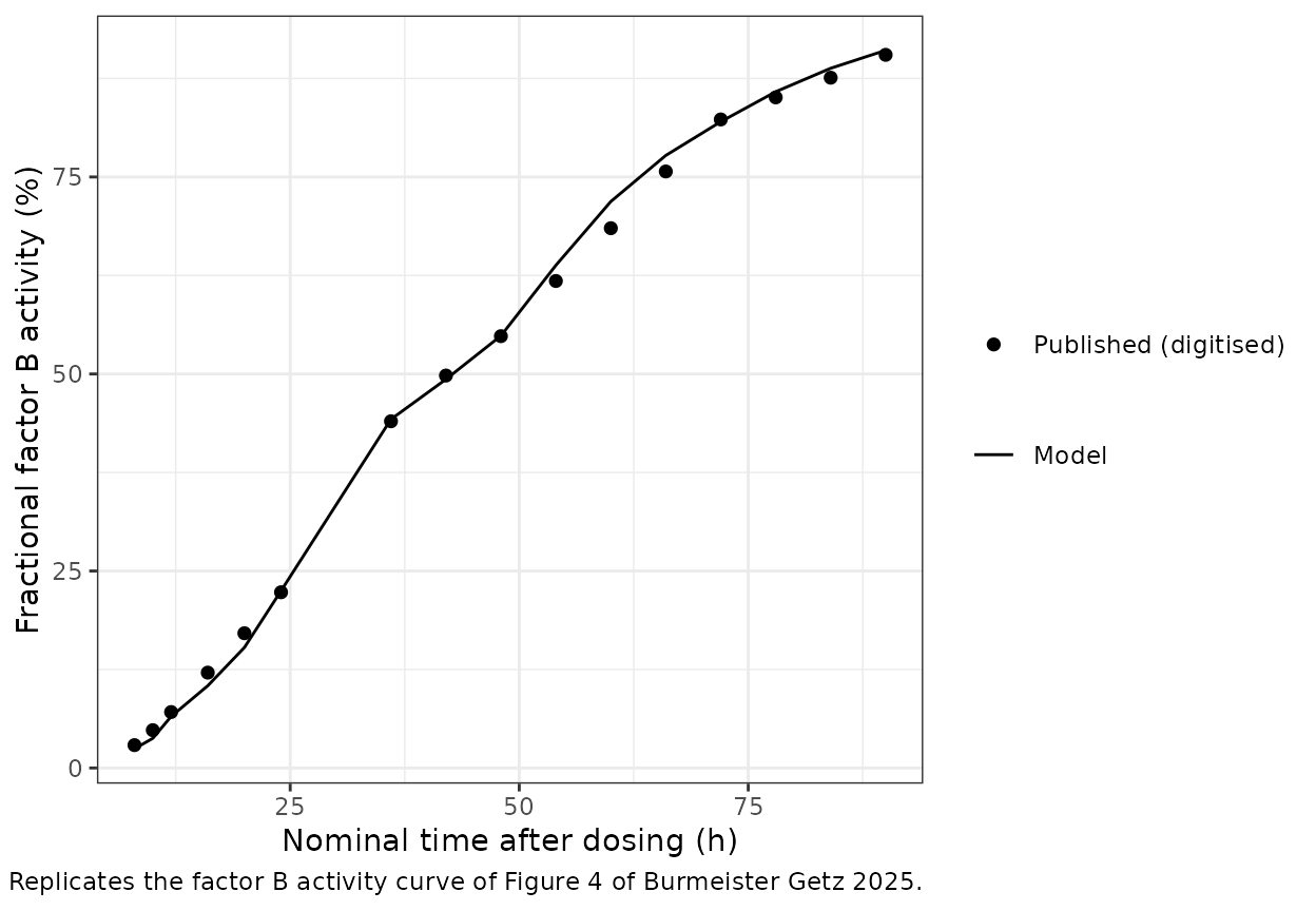
fig4 |>
  dplyr::select(time, total, unbound, unbound_model, unbound_pct_diff, activity, activity_model, activity_diff) |>
  dplyr::rename(
    "Time (h)" = time,
    "Total (ng/mL)" = total,
    "Unbound, published (ng/mL)" = unbound,
    "Unbound, model (ng/mL)" = unbound_model,
    "Unbound difference (%)" = unbound_pct_diff,
    "Activity, published (%)" = activity,
    "Activity, model (%)" = activity_model,
    "Activity difference (points)" = activity_diff
  ) |>
knitr::kable(digits = 2)| Time (h) | Total (ng/mL) | Unbound, published (ng/mL) | Unbound, model (ng/mL) | Unbound difference (%) | Activity, published (%) | Activity, model (%) | Activity difference (points) |
|---|---|---|---|---|---|---|---|
| 6 | 1773.0 | 253.00 | 248.46 | -1.80 | NA | 1.61 | NA |
| 8 | 1425.0 | 162.00 | 163.09 | 0.67 | 2.9 | 2.43 | -0.47 |
| 10 | 1178.0 | 90.80 | 103.97 | 14.51 | 4.8 | 3.77 | -1.03 |
| 12 | 973.0 | NA | 58.20 | NA | 7.1 | 6.53 | -0.57 |
| 16 | 849.0 | NA | 34.93 | NA | 12.1 | 10.43 | -1.67 |
| 20 | 761.0 | 23.20 | 22.54 | -2.84 | 17.1 | 15.29 | -1.81 |
| 24 | 670.0 | 14.00 | 14.03 | 0.21 | 22.3 | 22.48 | 0.18 |
| 36 | 462.0 | NA | 5.13 | NA | 44.0 | 44.25 | 0.25 |
| 42 | 418.0 | NA | 4.18 | NA | 49.8 | 49.33 | -0.47 |
| 48 | 371.0 | 3.38 | 3.35 | -0.89 | 54.8 | 54.84 | 0.04 |
| 54 | 296.0 | NA | 2.31 | NA | 61.8 | 63.79 | 1.99 |
| 60 | 229.0 | NA | 1.59 | NA | 68.5 | 71.89 | 3.39 |
| 66 | 181.0 | 1.20 | 1.17 | -2.87 | 75.7 | 77.73 | 2.03 |
| 72 | 146.0 | 0.88 | 0.89 | 1.40 | 82.3 | 82.01 | -0.29 |
| 78 | 115.0 | 0.70 | 0.67 | -3.94 | 85.1 | 85.82 | 0.72 |
| 84 | 90.8 | 0.51 | 0.51 | 0.69 | 87.6 | 88.79 | 1.19 |
| 90 | 72.3 | NA | 0.40 | NA | 90.5 | 91.07 | 0.57 |
Closed-form checks against the published numbers
The model is time-independent and has no dosing, so a PKNCA analysis has nothing to act on; the checks below replace it. Each compares a model output with a number printed in the paper.
Mass balance
Rebuilding total iptacopan from the model’s unbound concentration with the forward binding equation (Figure 2a) must return the input.
# The solved output also carries bmax / kd / fumax, so the tabulated values
# are joined under distinct names.
mb <- sim |>
  dplyr::mutate(group = as.character(group)) |>
  dplyr::left_join(
    dplyr::rename(par_tab, p_bmax = bmax, p_kd = kd, p_fumax = fumax),
    by = "group"
  ) |>
  dplyr::mutate(
    ctot_rebuilt = cu_nm + p_bmax * cu_nm / (p_kd + cu_nm) + cu_nm * (1 - p_fumax) / p_fumax,
    rel_err = abs(ctot_rebuilt / ctot_nm - 1)
  )
max(mb$rel_err)
#> [1] 5.295764e-13
stopifnot(max(mb$rel_err) < 1e-8)
EC50 and EC90 (Table 3)
Table 3 gives, per group, the total iptacopan concentrations at which 50% and 90% of available factor B is occupied. Evaluating each model at those concentrations should return occupancies of 0.50 and 0.90.
ec_pub <- data.frame(
  group = group_levels,
  EC50 = c(412.04, 389.43, 306.28, 193.57),
  EC90 = c(857.43, 804.09, 622.24, 403.04)
)
ec_chk <- dplyr::bind_rows(lapply(seq_len(nrow(ec_pub)), function(i) {
  s <- solve_group(models[[ec_pub$group[i]]], c(ec_pub$EC50[i], ec_pub$EC90[i]))
  data.frame(
    group = ec_pub$group[i],
    EC50 = ec_pub$EC50[i],
    occ_at_EC50 = s$occ[1],
    EC90 = ec_pub$EC90[i],
    occ_at_EC90 = s$occ[2]
  )
}))
ec_chk |>
  dplyr::rename(
    "Group" = group,
    "EC50, Table 3 (ng/mL)" = EC50,
    "Model occupancy at EC50" = occ_at_EC50,
    "EC90, Table 3 (ng/mL)" = EC90,
    "Model occupancy at EC90" = occ_at_EC90
  ) |>
knitr::kable(digits = 4)| Group | EC50, Table 3 (ng/mL) | Model occupancy at EC50 | EC90, Table 3 (ng/mL) | Model occupancy at EC90 |
|---|---|---|---|---|
| Healthy controls | 412.04 | 0.4998 | 857.43 | 0.8993 |
| Mild HI | 389.43 | 0.4999 | 804.09 | 0.8998 |
| Moderate HI | 306.28 | 0.4999 | 622.24 | 0.8995 |
| Severe HI | 193.57 | 0.4999 | 403.04 | 0.8997 |
Distribution of drug at the healthy EC90
The paper states that at the healthy-control EC90 of 857.43 ng/mL, 83.1% of iptacopan is bound to factor B, 12.6% to non-specific plasma proteins and 4.3% is unbound.
s90 <- solve_group(models[["Healthy controls"]], 857.43) |>
  dplyr::mutate(ctot_nm = CP_IPTACOPAN_NGML * 1000 / mw_iptacopan, cu_nm = Cu * 1000 / mw_iptacopan)
part <- data.frame(
  state = c("Bound to factor B", "Bound non-specifically", "Unbound"),
  published = c(83.1, 12.6, 4.3),
  model = 100 * c(
    p_h[["bmax"]] * s90$occ,
    s90$cu_nm * (1 - p_h[["fumax"]]) / p_h[["fumax"]],
    s90$cu_nm
  ) / s90$ctot_nm
)
part |>
  dplyr::rename("Binding state" = state, "Published (%)" = published, "Model (%)" = model) |>
knitr::kable(digits = 2)| Binding state | Published (%) | Model (%) |
|---|---|---|
| Bound to factor B | 83.1 | 83.06 |
| Bound non-specifically | 12.6 | 12.71 |
| Unbound | 4.3 | 4.24 |
Trough occupancy at 100 mg versus 200 mg twice daily
The paper reports that a 34% lower steady-state trough (100 mg vs 200 mg bid) lowers end-of-interval factor B occupancy from 96% to 83% at average exposure, and from 90% to 67% for exposures near the lower end of the population. The model reproduces this self-consistently: invert the 200 mg occupancy to a total trough, scale it by 0.66 and evaluate the 100 mg occupancy.
total_at_occ <- function(occ, p) {
  cu <- occ * p[["kd"]] / (1 - occ)
  (cu / p[["fumax"]] + p[["bmax"]] * occ) * mw_iptacopan / 1000
}
trough <- data.frame(
  exposure = c("Average", "Lower end"),
  occ_200 = c(0.96, 0.90),
  occ_100_published = c(0.83, 0.67)
) |>
  dplyr::mutate(trough_200 = sapply(occ_200, total_at_occ, p = p_h))
trough$occ_100_model <- solve_group(models[["Healthy controls"]], 0.66 * trough$trough_200)$occ
trough |>
  dplyr::rename(
    "Exposure" = exposure,
    "Occupancy at 200 mg bid trough" = occ_200,
    "Implied 200 mg trough (ng/mL)" = trough_200,
    "Occupancy at 100 mg bid, published" = occ_100_published,
    "Occupancy at 100 mg bid, model" = occ_100_model
  ) |>
knitr::kable(digits = 3)| Exposure | Occupancy at 200 mg bid trough | Occupancy at 100 mg bid, published | Implied 200 mg trough (ng/mL) | Occupancy at 100 mg bid, model |
|---|---|---|---|---|
| Average | 0.96 | 0.83 | 1150.863 | 0.846 |
| Lower end | 0.90 | 0.67 | 859.216 | 0.674 |
The published occupancies are rounded to whole percentages, which accounts for the 1-2 point difference at average exposure.
Unbound Cmax from total Cmax (Table 2)
Because the transform is monotone, each participant’s unbound Cmax is the model applied to their total Cmax. Applying the model to the geometric-mean total Cmax gives an approximation to the geometric-mean unbound Cmax; it is not exact, because the geometric mean of a nonlinear transform differs from the transform of the geometric mean and because the binding parameters vary between participants, which the group-level fit does not describe.
cmax <- data.frame(
  group = group_levels,
  cmax_total = c(3490, 3560, 3230, 3260), # Table 2 geometric means
  cmax_u_published = c(711, 905, 1070, 1450)
)
cmax$cmax_u_model <- sapply(seq_len(nrow(cmax)), function(i) {
  solve_group(models[[cmax$group[i]]], cmax$cmax_total[i])$Cu
})
cmax$pct_diff <- 100 * (cmax$cmax_u_model / cmax$cmax_u_published - 1)
cmax |>
  dplyr::rename(
    "Group" = group,
    "Total Cmax, geo-mean (ng/mL)" = cmax_total,
    "Unbound Cmax, geo-mean, published (ng/mL)" = cmax_u_published,
    "Unbound Cmax, model (ng/mL)" = cmax_u_model,
    "Difference (%)" = pct_diff
  ) |>
knitr::kable(digits = 1)| Group | Total Cmax, geo-mean (ng/mL) | Unbound Cmax, geo-mean, published (ng/mL) | Unbound Cmax, model (ng/mL) | Difference (%) |
|---|---|---|---|---|
| Healthy controls | 3490 | 711 | 675.7 | -5.0 |
| Mild HI | 3560 | 905 | 900.4 | -0.5 |
| Moderate HI | 3230 | 1070 | 897.4 | -16.1 |
| Severe HI | 3260 | 1450 | 1415.6 | -2.4 |
Healthy controls, mild HI and severe HI agree within 5%. Moderate HI is 16% low: that group’s unbound Cmax varies much more between participants (geometric CV 41.8%) than its total Cmax does (22.3%), which a single group-level binding curve cannot reproduce.
Assumptions and deviations
- Four files for four fits. The paper fitted the binding model separately to each hepatic-function group (Results, ‘Iptacopan PPB model’), so each group is its own model. Choose the file matching the population of interest; there is no covariate model linking the groups.
-
Total concentration is an input, not a PK model.
The paper publishes no structural iptacopan PK model. Supply
CP_IPTACOPAN_NGMLfrom observed concentrations or from an external iptacopan PK model. -
Fitting direction. The paper states the binding
model was fitted to the total and unbound concentrations with
minpack.lm::nlsLMand a proportional error model, but not which concentration was the response. The packaged model returnsCufromCtot(eq. 2), the direction the paper uses for occupancy; the parameter values are the same either way. -
Residual error. The magnitude of the proportional
error is not reported, so
propSdisfixed(0). The model gives deterministic predictions; it has no inter-individual variability because the source fit was a pooled per-group regression. -
Observation name
Cu. The single output is the unbound concentration. It keeps the nameCuused across the library for unbound plasma concentration rather thanCc, which would imply total drug. The conventions checker flags a single-outputCuas non-canonical; this is expected here. -
Units.
bmaxandkdare in nM as tabulated; the model converts total and unbound iptacopan between ng/mL and nM with the molecular weight 422.52 g/mol (Table 3 footnote b). The ug/mL figures for fB,avail in Table 3 assume a factor B molecular weight of 90 kDa. The Results text quotes 168.5 ug/mL for the healthy-control fB,avail, while Table 3 gives 168.69 ug/mL (1874.30 nM); the model uses the nM value. - Rounded fu,max. Table 3 gives fu,max to two decimals. Recomputing EC50 and EC90 from the tabulated parameters reproduces Table 3 within 0.25%, which is the residual effect of that rounding.
- Figure 4 digitisation. The Figure 4 points were read from the published image by the maintainers; the peak region (about 1-5 h) is hidden by the figure legend and was not used.