Metformin (Li 2020) • nlmixr2lib

Model and source

Citation: Li L, Guan Z, Li R, Zhao W, Hao G, Yan Y, Xu Y, Liao L, Wang H, Gao L, Wu K, Gao Y, Li Y. Population pharmacokinetics and dosing optimization of metformin in Chinese patients with type 2 diabetes mellitus. Medicine (Baltimore). 2020;99(46):e23212. doi:10.1097/MD.0000000000023212
Description: One-compartment population pharmacokinetic model with first-order oral absorption and an absorption-lag time for immediate-release metformin hydrochloride at steady state in Chinese adults with type 2 diabetes mellitus (Li 2020). Apparent oral clearance scales as a power function of body weight (reference 75 kg) and of CKD-EPI estimated glomerular filtration rate (reference 102.5 mL/min/1.73 m^2); between-subject variability is estimated on CL/F only. OCT1, OCT2 and MATE1 polymorphisms were screened and not retained.
Article: https://doi.org/10.1097/MD.0000000000023212 (open access, PMC7668473)

Population

Li 2020 enrolled 130 hospitalized Chinese adults with type 2 diabetes mellitus (1999 WHO criteria) at Shandong Provincial Qianfoshan Hospital, Jinan, between February and September 2017 (ChiCTR1800014273). All had taken immediate-release metformin hydrochloride (Glucophage film-coated tablets) for at least 7 days, so sampling was at pharmacokinetic steady state. Five patients were excluded for irregular regimens or non-adherence, leaving 125 (85 male / 40 female) with 160 plasma samples (1-2 per patient, aimed at the 2-4 h peak and the 10-12 h trough). Median (range) age was 56 (27-83) years, body weight 75 (51-113) kg, BMI 26.4 (18.1-35.3) kg/m^2 and CKD-EPI eGFR 102.5 (46.9-137.7) mL/min/1.73 m^2 (Table 1). Regimens were 1000 mg b.i.d. (n = 55), 500 mg t.i.d. (n = 29), 500 mg b.i.d. (n = 28), 500 mg q.i.d. (n = 12) and 850 mg q.d. (n = 1) (Results section 3.1). Table 2 splits the cohort into eGFR strata of 45-59, 60-89, 90-120 and >= 120 mL/min/1.73 m^2 (5, 26, 73 and 10 patients).

The same information is available programmatically via readModelDb("Li_2020_metformin")()$population.

Source trace

The per-parameter origin is recorded as an in-file comment next to each ini() entry in inst/modeldb/specificDrugs/Li_2020_metformin.R. The table below collects them in one place for review.

Equation / parameter	Value	Source location
Structural model	1-compartment, first-order absorption with lag time	Results section 3.3; Discussion paragraph 1
`lka` = log(1.4)	1.4 1/h	Table 4, ka (RSE 51.5%)
`lcl` = log(53.0)	53.0 L/h	Table 4, theta1 (RSE 4.6%); final CL/F equation, Results section 3.4
`lvc` = log(438)	438 L	Table 4, V/F (RSE 15.0%); Results section 3.4
`ltlag` = log(0.914)	0.914 h	Table 4, tlag (RSE 30.3%)
`e_wt_cl`	0.688	Table 4, theta2 (RSE 24.6%)
`e_crcl_cl`	0.914	Table 4, theta3 (RSE 19.9%)
CL/F = theta1 (WT/75)^theta2 (eGFR/102.5)^theta3 exp(eta)	n/a	Table 4 row header; Results section 3.4; abstract
`etalcl` variance	0.0323	Table 4 IIV CL/F 18.0%; eta term printed as EXP(0.1797) in the CL/F equation (0.1797^2 = 0.0323)
`propSd`	0.3507	Table 4, residual variability 35.07% (exponential model, Results section 3.3)
Reference WT = 75 kg, eGFR = 102.5	n/a	Table 1 cohort medians, used as the equation’s normalisers

Deterministic checks against reported values

The Results report a median (range) individual weight-normalised CL/F of 0.71 (0.31-0.99) L/h/kg (section 3.4). A typical 75 kg patient at the reference eGFR has CL/F/WT = 53.0/75 = 0.707 L/h/kg, which reproduces the median. The printed CL/F equation also carries a literal EXP(0.1797) term; read as a fixed multiplier it would raise the typical CL/F to 53.0 x 1.197 = 63.4 L/h and the median to 0.85 L/h/kg, contradicting both this median and the abstract’s “apparent clearance 53.0 L/h”. The term is therefore the eta, written with its standard deviation (see Assumptions).

mod <- readModelDb("Li_2020_metformin")
mod_typ <- mod |> rxode2::zeroRe()
th <- rxode2::rxode(mod)$theta

typ_cl <- function(wt, crcl) {
  exp(th[["lcl"]]) * (wt / 75)^th[["e_wt_cl"]] * (crcl / 102.5)^th[["e_crcl_cl"]]
}

cl_ref <- typ_cl(75, 102.5)
cl_per_kg_ref <- cl_ref / 75
cl_literal_multiplier <- cl_ref * exp(0.1797) / 75

knitr::kable(
  data.frame(
    Quantity = c(
      "Typical CL/F at WT 75 kg, eGFR 102.5 (L/h)",
      "Typical CL/F / WT (L/h/kg)",
      "Reported median individual CL/F / WT (L/h/kg)",
      "CL/F / WT if EXP(0.1797) were a fixed multiplier (L/h/kg)"
    ),
    Value = signif(c(cl_ref, cl_per_kg_ref, 0.71, cl_literal_multiplier), 3)
  ),
  caption = "Reference-point checks against Li 2020 Results section 3.4."
)

Reference-point checks against Li 2020 Results section 3.4.
Quantity	Value
Typical CL/F at WT 75 kg, eGFR 102.5 (L/h)	53.000
Typical CL/F / WT (L/h/kg)	0.707
Reported median individual CL/F / WT (L/h/kg)	0.710
CL/F / WT if EXP(0.1797) were a fixed multiplier (L/h/kg)	0.846


stopifnot(
  abs(cl_ref - 53.0) < 1e-8,
  abs(cl_per_kg_ref / 0.71 - 1) < 0.01,
  abs(cl_literal_multiplier / 0.71 - 1) > 0.15
)

Virtual cohort

Original observed data are not publicly available. The virtual cohort keeps the paper’s regimen mix exactly (125 patients). Body weight is drawn from a normal distribution centred on the median 75 kg (SD 12 kg, an assumption) and redrawn until it falls in the observed 51-113 kg range. eGFR is drawn by first picking a Table 2 stratum in proportion to its size (5 / 26 / 73 / 10) and then drawing uniformly within that stratum’s observed range. Weight and eGFR are drawn independently.

# set.seed() fixes R's draws (covariates); rxode2's eta draws are partitioned
# per solver thread, so every assertion below holds for any cohort.
set.seed(20200716)
rxode2::rxSetSeed(20200716)

regimens <- tibble::tribble(
  ~treatment,      ~dose, ~tau, ~n,
  "1000 mg b.i.d.", 1000,   12, 55L,
  "500 mg t.i.d.",   500,    8, 29L,
  "500 mg b.i.d.",   500,   12, 28L,
  "500 mg q.i.d.",   500,    6, 12L,
  "850 mg q.d.",     850,   24,  1L
)
stopifnot(sum(regimens$n) == 125L)

egfr_strata <- tibble::tribble(
  ~lo,   ~hi,   ~n,
  46.9,  55.4,  5,
  60.6,  89.0,  26,
  90.1,  119.0, 73,
  120.4, 137.7, 10
)

draw_truncnorm <- function(n, mean, sd, lo, hi) {
  x <- rnorm(n, mean, sd)
  bad <- x < lo | x > hi
  while (any(bad)) {
    x[bad] <- rnorm(sum(bad), mean, sd)
    bad <- x < lo | x > hi
  }
  x
}

draw_egfr <- function(n) {
  s <- sample(seq_len(nrow(egfr_strata)), n, replace = TRUE, prob = egfr_strata$n)
  runif(n, egfr_strata$lo[s], egfr_strata$hi[s])
}

subjects <- regimens |>
  tidyr::uncount(n) |>
  mutate(
    id = seq_len(dplyr::n()),
    WT = draw_truncnorm(dplyr::n(), 75, 12, 51, 113),
    CRCL = draw_egfr(dplyr::n())
  )

# Steady state: one ss = 1 dose at time 0, then the full dosing interval
# observed densely on the central compartment.
dose_rows <- subjects |>
  mutate(time = 0, amt = dose, ii = tau, ss = 1L, evid = 1L, cmt = "depot")
obs_rows <- subjects |>
  group_by(id) |>
  reframe(
    treatment = treatment, dose = dose, tau = tau, WT = WT, CRCL = CRCL,
    time = seq(0, tau, by = 0.05)
  ) |>
  mutate(amt = NA_real_, ii = 0, ss = 0L, evid = 0L, cmt = "central")

events <- bind_rows(dose_rows, obs_rows) |>
  arrange(id, time, desc(evid)) |>
  select(id, time, evid, amt, ii, ss, cmt, WT, CRCL, treatment, dose, tau)

stopifnot(!anyDuplicated(events[, c("id", "time", "evid")]))

Simulation

sim <- rxode2::rxSolve(
  mod,
  events = events,
  keep = c("treatment", "dose", "tau", "WT", "CRCL"),
  rtol = 1e-10, atol = 1e-12, ssRtol = 1e-10, ssAtol = 1e-12,
  maxsteps = 1e6,
  returnType = "data.frame"
)
stopifnot(!anyNA(sim$Cc))

Individual clearance

ind <- sim |>
  distinct(id, treatment, dose, tau, WT, CRCL, cl) |>
  mutate(cl_per_kg = cl / WT, auc24_expected = dose * 24 / tau / cl)

summary(ind$cl_per_kg)
#>    Min. 1st Qu.  Median    Mean 3rd Qu.    Max. 
#>  0.3162  0.5501  0.6463  0.6690  0.7737  1.1690

# Median individual CL/F/WT is reported as 0.71 L/h/kg. The cohort median is
# a covariate-distribution statistic, not an extreme, so a 10% band is robust
# to the draw yet breaks on a mis-scaled clearance or exponent.
stopifnot(abs(median(ind$cl_per_kg) / 0.71 - 1) < 0.10)

Replicate published figures

Figure 1 of Li 2020 shows the 160 observed concentrations (0.22-4.01 mg/L) against time after dose, pooled across regimens. The ribbon below is the simulated 5th-95th percentile band of the same pooled cohort at steady state, with the observed range drawn as dashed lines.

sim |>
  mutate(tad_bin = round(time * 2) / 2) |>
  filter(tad_bin <= 12) |>
  group_by(tad_bin) |>
  summarise(
    Q05 = quantile(Cc, 0.05), Q50 = median(Cc), Q95 = quantile(Cc, 0.95),
    .groups = "drop"
  ) |>
  ggplot(aes(tad_bin, Q50)) +
  geom_ribbon(aes(ymin = Q05, ymax = Q95), alpha = 0.25) +
  geom_line() +
  geom_hline(yintercept = c(0.22, 4.01), linetype = "dashed") +
  labs(
    x = "Time after dose (h)", y = "Metformin plasma concentration (mg/L)",
    caption = "Replicates Figure 1 of Li 2020 (dashed: observed range 0.22-4.01 mg/L)."
  )

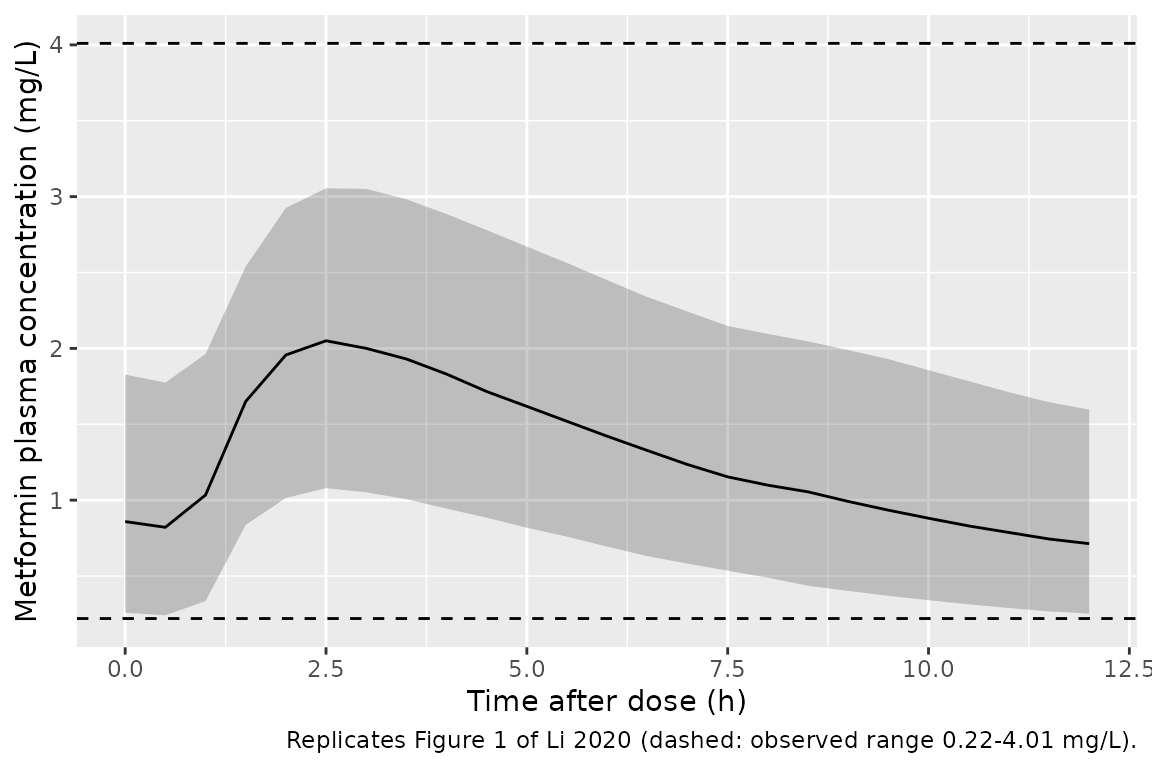
# Medians in the paper's two sampling windows sit inside the observed range.
win <- sim |>
  mutate(window = case_when(
    time >= 2 & time <= 4 ~ "peak (2-4 h)",
    time >= 10 & time <= 12 ~ "trough (10-12 h)"
  )) |>
  filter(!is.na(window)) |>
  group_by(window) |>
  summarise(median_Cc = median(Cc), .groups = "drop")
knitr::kable(win, digits = 2, caption = "Simulated median concentration in each sampling window.")

Simulated median concentration in each sampling window.
window	median_Cc
peak (2-4 h)	1.96
trough (10-12 h)	0.80

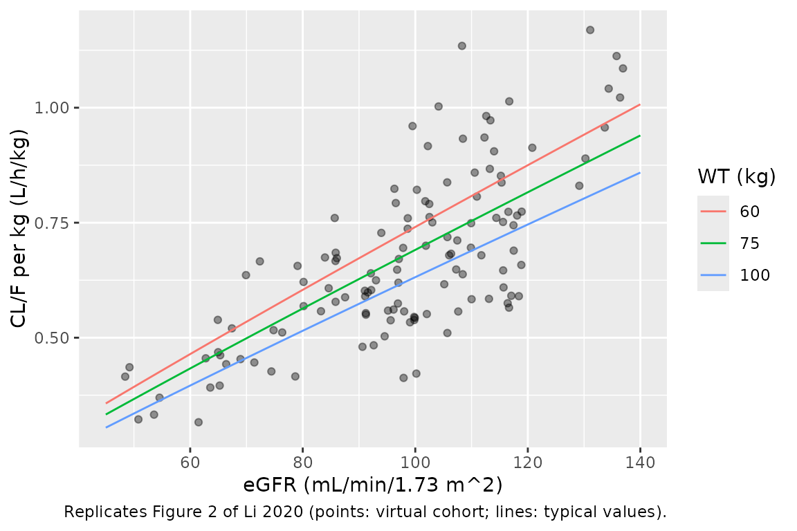
stopifnot(nrow(win) == 2L, all(win$median_Cc > 0.22 & win$median_Cc < 4.01))

Figure 2 of Li 2020 plots individual CL/F per kg against eGFR and shows a roughly proportional rise. The typical-value curves below are drawn at 60, 75 and 100 kg over the observed eGFR range, with the virtual cohort overlaid.

curves <- tidyr::crossing(WT = c(60, 75, 100), CRCL = seq(45, 140, by = 1)) |>
  mutate(cl_per_kg = typ_cl(WT, CRCL) / WT, WT = factor(WT))
ggplot() +
  geom_point(data = ind, aes(CRCL, cl_per_kg), alpha = 0.4) +
  geom_line(data = curves, aes(CRCL, cl_per_kg, colour = WT)) +
  labs(
    x = "eGFR (mL/min/1.73 m^2)", y = "CL/F per kg (L/h/kg)", colour = "WT (kg)",
    caption = "Replicates Figure 2 of Li 2020 (points: virtual cohort; lines: typical values)."
  )

PKNCA validation

NCA is run on the steady-state dosing interval of each simulated patient, grouped by regimen. AUC over one interval is scaled to 24 h to compare with the paper’s reported AUC0-24 range.

sim_nca <- sim |>
  filter(!is.na(Cc)) |>
  select(id, time, Cc, treatment)

# Every subject already has its time-zero (pre-dose trough) observation; the
# bind_rows + distinct guard keeps that true if the grid is ever changed.
sim_nca <- bind_rows(
  sim_nca,
  sim |> filter(time == 0) |> distinct(id, treatment, .keep_all = TRUE) |>
    select(id, time, Cc, treatment)
) |>
  distinct(id, treatment, time, .keep_all = TRUE) |>
  arrange(id, treatment, time)

conc_obj <- PKNCA::PKNCAconc(sim_nca, Cc ~ time | treatment + id)
dose_obj <- PKNCA::PKNCAdose(
  events |> filter(evid == 1) |> select(id, time, amt, treatment),
  amt ~ time | treatment + id
)
intervals <- regimens |>
  transmute(treatment, start = 0, end = tau, cmax = TRUE, cmin = TRUE, tmax = TRUE, auclast = TRUE)

nca_res <- PKNCA::pk.nca(PKNCA::PKNCAdata(conc_obj, dose_obj, intervals = as.data.frame(intervals)))

nca_wide <- as.data.frame(nca_res) |>
  select(treatment, id, PPTESTCD, PPORRES) |>
  tidyr::pivot_wider(names_from = PPTESTCD, values_from = PPORRES) |>
  left_join(ind |> select(id, tau, auc24_expected), by = "id") |>
  mutate(auc24 = auclast * 24 / tau)

nca_wide |>
  group_by(treatment) |>
  summarise(
    n = dplyr::n(),
    cmax = median(cmax), cmin = median(cmin), tmax = median(tmax),
    auc24 = median(auc24), .groups = "drop"
  ) |>
  dplyr::rename(
    Regimen = treatment, N = n, "Median Cmax (mg/L)" = cmax,
    "Median Cmin (mg/L)" = cmin, "Median Tmax (h)" = tmax,
    "Median AUC0-24 (mg*h/L)" = auc24
  ) |>
  knitr::kable(digits = 2, caption = "Simulated steady-state NCA by regimen.")

Simulated steady-state NCA by regimen.
Regimen	N	Median Cmax (mg/L)	Median Cmin (mg/L)	Median Tmax (h)	Median AUC0-24 (mg*h/L)
1000 mg b.i.d.	55	2.61	0.93	2.65	42.29
500 mg b.i.d.	28	1.30	0.46	2.65	21.03
500 mg q.i.d.	12	2.09	1.39	2.35	43.04
500 mg t.i.d.	29	1.61	0.85	2.45	30.39
850 mg q.d.	1	1.49	0.04	2.65	11.68

# Same drawn parameters on both sides: the trapezoidal AUC over a 0.05 h grid
# must equal Dose * (24 / tau) / CL up to numerical error only.
auc_err <- nca_wide$auc24 / nca_wide$auc24_expected - 1
stopifnot(nrow(nca_wide) == 125L, max(abs(auc_err)) < 0.005)

auc_range <- range(nca_wide$auc24)
knitr::kable(
  data.frame(
    Source = c("Li 2020 Results section 3.4 (individual estimates)", "Virtual cohort"),
    "Min AUC0-24" = c(12.35, auc_range[1]),
    "Max AUC0-24" = c(71.23, auc_range[2]),
    check.names = FALSE
  ),
  digits = 2,
  caption = "Steady-state AUC0-24 (mg*h/L) range."
)

Steady-state AUC0-24 (mg*h/L) range.
Source	Min AUC0-24	Max AUC0-24
Li 2020 Results section 3.4 (individual estimates)	12.35	71.23
Virtual cohort	11.48	74.25

# The median sits inside the published range; the extremes are draw-dependent
# and are displayed, not asserted.
stopifnot(median(nca_wide$auc24) > 12.35, median(nca_wide$auc24) < 71.23)

Comparison against published NCA

Li 2020 reports no central NCA values (no Cmax, Cmin or AUC by regimen), only the AUC0-24 range of the individual estimates shown above, so no ncaComparisonTable() is rendered.

Dosing recommendations (Table 5)

Li 2020 chose, for each eGFR stratum, the smallest regimen at which the simulated 95th percentile of steady-state Cmax stayed below 5 mg/L and the 5th percentile of Cmin stayed above 0.4 mg/L (Methods section 2.6). The Table 5 values are total daily doses: 2550 mg/day t.i.d. and 3000 mg/day b.i.d. for augmented renal clearance, as the abstract and Discussion state.

The percentiles are reproduced deterministically here. Both Cmax and Cmin fall monotonically with CL/F, and CL/F carries the model’s only eta, so at fixed covariates the 5th percentile of Cmin is the solve at eta = +1.645 omega and the 95th percentile of Cmax is the solve at eta = -1.645 omega. Covariates are the Table 2 stratum medians. Residual error is excluded, since the criterion concerns true concentrations.

omega_sd <- sqrt(rxode2::rxode(mod)$omega["etalcl", "etalcl"])

table5 <- tibble::tribble(
  ~stage,  ~egfr_label, ~WT,  ~CRCL,  ~daily8, ~daily12,
  "G3a",   "45-59",     71.5, 50.4,   750,     1000,
  "G2",    "60-89",     75,   79.7,   1275,    1700,
  "G1",    "90-119",    75,   105,    1500,    2000,
  "ARC",   ">=120",     87,   123.7,  2550,    3000
) |>
  tidyr::pivot_longer(c(daily8, daily12), names_to = "interval", values_to = "daily_dose") |>
  mutate(tau = ifelse(interval == "daily8", 8, 12), dose = daily_dose * tau / 24)

make_q_events <- function(tbl, eta) {
  subj <- tbl |> mutate(id = seq_len(dplyr::n()), etalcl = eta)
  ev <- bind_rows(
    subj |> mutate(time = 0, amt = dose, ii = tau, ss = 1L, evid = 1L, cmt = "depot"),
    subj |>
      group_by(id) |>
      reframe(WT = WT, CRCL = CRCL, tau = tau, time = seq(0, tau, by = 0.01)) |>
      mutate(amt = NA_real_, ii = 0, ss = 0L, evid = 0L, cmt = "central")
  ) |>
    arrange(id, time, desc(evid)) |>
    select(id, time, evid, amt, ii, ss, cmt, WT, CRCL)
  list(ev = ev, params = subj |> select(id, etalcl))
}

solve_q <- function(tbl, eta) {
  q <- make_q_events(tbl, eta)
  rxode2::rxSolve(
    mod_typ, events = q$ev, params = q$params,
    rtol = 1e-10, atol = 1e-12, ssRtol = 1e-10, ssAtol = 1e-12,
    maxsteps = 1e6, returnType = "data.frame"
  ) |>
    group_by(id) |>
    summarise(cmax = max(Cc), cmin = min(Cc), .groups = "drop")
}

hi <- solve_q(table5, -qnorm(0.95) * omega_sd) # low CL -> 95th pct Cmax
#> Warning: multi-subject simulation without without 'omega'
lo <- solve_q(table5, qnorm(0.95) * omega_sd)  # high CL -> 5th pct Cmin
#> Warning: multi-subject simulation without without 'omega'
t5 <- table5 |>
  mutate(id = seq_len(dplyr::n()), p95_cmax = hi$cmax, p5_cmin = lo$cmin)

# Alternative reading: Table 5 values as per-administration doses.
per_admin <- solve_q(table5 |> mutate(dose = daily_dose), -qnorm(0.95) * omega_sd)
#> Warning: multi-subject simulation without without 'omega'
t5$p95_cmax_per_admin <- per_admin$cmax

t5 |>
  transmute(
    stage, egfr_label, interval = paste0("q", tau, "h"), daily_dose, dose,
    p95_cmax, p5_cmin, p95_cmax_per_admin
  ) |>
  dplyr::rename(
    Stage = stage, "eGFR (mL/min/1.73 m^2)" = egfr_label, Interval = interval,
    "Daily dose (mg)" = daily_dose, "Dose per administration (mg)" = dose,
    "P95 Cmax (mg/L)" = p95_cmax, "P5 Cmin (mg/L)" = p5_cmin,
    "P95 Cmax if Table 5 were per administration (mg/L)" = p95_cmax_per_admin
  ) |>
  knitr::kable(digits = 2, caption = "Reproduction of Li 2020 Table 5 at stratum-median covariates.")

Reproduction of Li 2020 Table 5 at stratum-median covariates.
Stage	eGFR (mL/min/1.73 m^2)	Interval	Daily dose (mg)	Dose per administration (mg)	P95 Cmax (mg/L)	P5 Cmin (mg/L)	P95 Cmax if Table 5 were per administration (mg/L)
G3a	45-59	q8h	750	250	1.73	0.65	5.20
G3a	45-59	q12h	1000	500	2.49	0.72	4.98
G2	60-89	q8h	1275	425	1.98	0.59	5.95
G2	60-89	q12h	1700	850	2.96	0.58	5.91
G1	90-119	q8h	1500	500	1.89	0.47	5.68
G1	90-119	q12h	2000	1000	2.90	0.41	5.80
ARC	>=120	q8h	2550	850	2.64	0.51	7.92
ARC	>=120	q12h	3000	1500	3.69	0.34	7.37

stopifnot(nrow(t5) == 8L)
# Upper criterion: met in every cell under the daily-dose reading...
stopifnot(all(t5$p95_cmax < 5))
# ...and violated under the per-administration reading, which rules it out.
stopifnot(any(t5$p95_cmax_per_admin > 5))
# Lower criterion: met everywhere except ARC q12h (see Assumptions).
arc12 <- t5$stage == "ARC" & t5$tau == 12
# Deterministic (no draws): measured 0.41-0.72 for the seven cells and 0.34
# for ARC q12h.
stopifnot(all(t5$p5_cmin[!arc12] > 0.4), t5$p5_cmin[arc12] < 0.4)
stopifnot(sum(t5$p95_cmax_per_admin > 5) == 7L)

The daily-dose reading keeps the 95th percentile of Cmax below 5 mg/L in every cell; read as per-administration doses, seven of the eight cells exceed it. The 5th percentile of Cmin is above 0.4 mg/L in seven of the eight cells, and the G1 cells sit close to the threshold (about 0.47 and 0.41 mg/L), as a minimum-dose search would produce. The exception is ARC at 1500 mg q12h (about 0.34 mg/L at the stratum median), where the recommendation is not reproduced; see Assumptions.

Assumptions and deviations

The EXP(0.1797) term in the CL/F equation. Table 4, the Results and the abstract all print CL/F = 53.0 (WT/75)^0.688 (eGFR/102.5)^0.914 EXP(0.1797). Read literally, the constant would multiply the typical CL/F by 1.197. It is interpreted as the eta term written with its standard deviation: 0.1797 equals the Table 4 IIV of 18.0% to rounding, the abstract gives the population CL/F as 53.0 L/h, and the reported median CL/F/WT of 0.71 L/h/kg matches 53.0/75 = 0.707 but not 63.4/75 = 0.85 (checked above). The between-subject variance is therefore omega^2 = 0.1797^2 = 0.0323.
Residual error. The paper describes an exponential residual model with 35.07% variability (Results section 3.3, Table 4). It is encoded as proportional error with propSd = 0.3507, the first-order equivalent of NONMEM Y = F * EXP(EPS).
Dose units. Doses are metformin hydrochloride as labelled (Glucophage tablets). The paper does not state whether concentrations are reported as the base or the salt; CL/F and V/F are apparent parameters for the labelled hydrochloride dose, so use hydrochloride doses with this model.
No IIV on V/F, ka or tlag. Only CL/F carried IIV in the final model (Results section 3.3); with 1-2 samples per patient the absorption parameters were poorly determined (ka RSE 51.5%).
Virtual cohort. The body-weight SD (12 kg) is assumed; the paper gives only the median and range. Weight and eGFR are drawn independently, whereas in the source cohort the ARC stratum was heavier and younger (Table 2). The Table 2 stratum counts sum to 114, not 125; they are used as relative weights.
Table 5 reproduction. Li 2020 ran 1000 replicate simulations of the original dataset (5 to 73 patients per stratum), which is not available. The reproduction above uses deterministic percentiles at stratum-median covariates, excluding residual error. Seven of eight cells meet both criteria; ARC at 3000 mg/day b.i.d. gives a 5th-percentile Cmin of about 0.34 mg/L rather than above 0.4 mg/L. The model parameters are not adjusted to close this gap. The likely cause is the paper’s simulation method (the specific ARC patients, and whether residual error or covariate spread entered the percentiles), which the paper does not describe in enough detail to replicate.
Genetic and demographic covariates not retained. Age, BMI and the OCT1 rs622342, OCT2 rs316019 and MATE1 rs2289669 / rs2252281 variants were screened on CL/F and dropped (delta OFV < 3.84). They are recorded in the model’s covariatesDataExcluded metadata.
Errata. No erratum or correction for this article was found in the EuropePMC record (checked 2026-09-27).