Meropenem (Braune 2018)
Source:vignettes/articles/Braune_2018_meropenem.Rmd
Braune_2018_meropenem.RmdModel and source
#> ℹ parameter labels from comments will be replaced by 'label()'Citation: Braune S, Konig C, Roberts JA, Nierhaus A, Steinmetz O, Baehr M, Kluge S, Langebrake C. Pharmacokinetics of meropenem in septic patients on sustained low-efficiency dialysis: a population pharmacokinetic study. Crit Care. 2018;22(1):25. doi:10.1186/s13054-018-1940-1
Description: Two-compartment IV population PK model for meropenem in 19 septic critically ill adults with acute kidney injury receiving sustained low-efficiency dialysis (Braune 2018). Pmetrics NPAG non-parametric fit parameterised by a central volume and the rate constants Kcp / Kpc. Total clearance is the additive sum of three arms: a non-renal arm (2.6 L/h), a native renal arm proportional to 24-hour residual diuresis (1.5 L/h per 100 mL/24h), and a SLED arm (7.9 L/h) switched on only while a dialysis session is running. Blood/dialysate flow, ultrafiltration rate and body weight were screened but not retained.
PubMed Central: https://www.ncbi.nlm.nih.gov/pmc/articles/PMC5791175/
Braune 2018 is a prospective single-centre population PK study of meropenem in critically ill septic adults with acute kidney injury who were receiving sustained low-efficiency dialysis (SLED), a prolonged-intermittent renal replacement modality. The clinically interesting feature – and the reason the model is worth packaging – is that meropenem clearance is not a single number: it switches between a low interdialytic value and a much higher intradialytic value every time a SLED session starts and stops, and the interdialytic value itself depends on how much urine the patient still makes.
Population
19 septic adults (73.7% male) contributed 308 serum meropenem concentrations. Median age was 66 years [range 37-78], median weight 81 kg [range 70-183], and median SOFA score on the first sampling day 11 [range 5-16]. All were on SLED for acute kidney injury; the median residual diuresis was 0 mL/24h, i.e. the median patient was anuric, with an interquartile range of 0-80 mL/24h and a maximum of 360 mL/24h (Braune 2018 Table 1). ICU mortality was 47%.
Meropenem was given as 0.5 g, 1 g or 2 g IV over 30 minutes 8-hourly at the discretion of the treating physician. Sampling ran over three consecutive SLED days: a trough 1 h before the infusion, then 10 min, 1 h, 2 h and 4 h after the start of SLED, and at the end of the session. Post-SLED samples were not collected, so any post-dialysis rebound is unobserved (Braune 2018 Limitations).
The same information is available programmatically via
readModelDb("Braune_2018_meropenem")()$population.
Source trace
Every ini() entry carries an in-file comment naming its
source location; the table below collects them for review. All parameter
values come from Table 2 (“Parameter estimates for
meropenem from the final covariate two-compartment population
pharmacokinetic model”), whose columns are Mean / Standard deviation /
Coefficient of variation (%) / Median. The typical values below are the
Mean column – the column the Discussion quotes
throughout.
| Equation / parameter | Value | Source location |
|---|---|---|
lcl_nonren (CLD) |
log(2.6) L/h |
Table 2, row CLD: mean 2.6, SD 1.2, CV 44.9%, median
2.3 |
lcl_renal (CLN) |
log(1.5) L/h per 100 mL/24h |
Table 2, row CLN: mean 1.5, SD 2.1, CV 134.7%, median
0.7 |
lcl_crrt (CLSLED) |
log(7.9) L/h |
Table 2, row CLSLED: mean 7.9, SD 4.2, CV 53.6%, median
6.8 |
lvc (Vc) |
log(8.1) L |
Table 2, row Vc: mean 8.1, SD 7.1, CV 87.9%, median
4.9 |
lk12 (Kcp) |
log(10.3) 1/h |
Table 2, row KCP: mean 10.3, SD 8.8, CV 85.4%, median
7.9 |
lk21 (Kpc) |
log(1.8) 1/h |
Table 2, row KPC: mean 1.8, SD 1.9, CV 104.4%, median
1.2 |
etalcl_nonren … etalk21
|
log(CV^2 + 1) |
Table 2, “Coefficient of variation (%)” column |
addSd |
fixed(0) |
Methods / Results state an additive (lambda) error model; the magnitude is reported nowhere |
cl <- cl_nonren + cl_renal + RRT_CRRT_ACTIVE * cl_crrt |
n/a | Results, “Pharmacokinetic model building”:
TVCL = CLSLED * (SLED) + CLNS
|
cl_renal <- exp(lcl_renal + eta) * URINE_VOL_24H / 100 |
n/a | Same equation block:
TVCLNS = CLD + (CLN * RD / 100)
|
| Two-compartment ODEs in Kcp / Kpc | n/a | Table 2 parameterisation; Abbreviations list defines KCP / KPC |
| SLED indicator semantics | 1 on / 0 off | Results: “The value for term SLED is 1 when SLED is on, whereas it is 0 when SLED is off” |
The two model equations are printed in the article as a single
typeset image. The PDF text layer silently drops the multiplication
signs from that image (TVCL = CLSLED (SLED) + CLNS), which
reads ambiguously; the publisher’s figure-file bundle for PMC5791175
contains the image itself
(13054_2018_1940_Article_Equa.gif), which renders
unambiguously as TVCL = CL_SLED * (SLED) + CL_NS. The SLED
arm is therefore additive on top of the interdialytic
arms, not a replacement for them. See “Assumptions and deviations” for
the one Discussion sentence that reads loosely against this.
Structural verification
These checks compare the packaged model against quantities that follow algebraically from the published parameters. They are deterministic – typical values with the random effects zeroed – so the difference between the two sides is pure numerical error and a tight bound is the correct gate.
mod <- readModelDb("Braune_2018_meropenem")
mod_typical <- rxode2::zeroRe(rxode2::rxode(mod))
#> ℹ parameter labels from comments will be replaced by 'label()'

# Published parameters (Braune 2018 Table 2, Mean column).
p <- list(cld = 2.6, cln = 1.5, clsled = 7.9, vc = 8.1, kcp = 10.3, kpc = 1.8)

# The paper's printed clearance equation, evaluated directly.
published_cl <- function(rd, sled) p$clsled * sled + p$cld + p$cln * rd / 100

# Build an event table. `rate` (not `dur`) sets the infusion duration explicitly.
# RRT_CRRT_ACTIVE is time-varying, so it is supplied on EVERY record and the
# solve below uses covsInterpolation = "locf" -- linear interpolation would ramp
# a binary on/off gate across the transition instead of switching it.
make_events <- function(n, dose_mg, ii = 8, n_doses = 1L, rd = 0,
                        sled_start = NA_real_, sled_dur = 5, infusion_h = 0.5,
                        tmax = 48, dt = 0.1, id_offset = 0L) {
  dose_times <- seq(0, by = ii, length.out = n_doses)
  sled_edges <- if (is.na(sled_start)) numeric(0) else c(sled_start, sled_start + sled_dur)
  obs_times <- sort(unique(c(
    seq(0, tmax, by = dt),
    # resolve the fast distribution phase (alpha half-life ~3 min) after each dose
    as.vector(outer(dose_times, c(seq(0, infusion_h, by = 0.02), seq(0.6, 2, by = 0.05)), "+")),
    dose_times, dose_times + infusion_h, sled_edges
  )))
  obs_times <- obs_times[obs_times >= 0 & obs_times <= tmax]
  one <- dplyr::bind_rows(
    dplyr::tibble(time = dose_times, evid = 1L, amt = dose_mg,
                  rate = dose_mg / infusion_h, cmt = "central"),
    dplyr::tibble(time = obs_times, evid = 0L, amt = NA_real_,
                  rate = NA_real_, cmt = "central")
  ) |>
    dplyr::arrange(.data$time, dplyr::desc(.data$evid))
  tidyr::expand_grid(id = id_offset + seq_len(n), one) |>
    dplyr::mutate(
      URINE_VOL_24H = rd,
      RRT_CRRT_ACTIVE =
        if (is.na(sled_start)) 0 else
          as.numeric(.data$time >= sled_start & .data$time < sled_start + sled_dur)
    )
}

solve_typical <- function(events, ...) {
  rxode2::rxSolve(mod_typical, events, covsInterpolation = "locf",
                  returnType = "data.frame", ...)
}
1. The published clearance equation is reproduced exactly
For a linear model given intravenously,
CL * AUC(0-Inf) == Dose identically. Recovering the paper’s
own TVCL from the simulated AUC therefore tests the whole
covariate equation – both arms of the interdialytic clearance, the
RD / 100 normalisation, and the additive SLED gate – in one
number.
grid_cl <- tidyr::expand_grid(rd = c(0, 100, 300), sled = c(0, 1))

cl_check <- grid_cl |>
  rowwise() |>
  mutate(
    sim = list({
      # SLED held constant for the whole profile so a single CL applies.
      ev <- make_events(1, dose_mg = 1000, rd = .data$rd, tmax = 240, dt = 0.05,
                        sled_start = if (.data$sled == 1) 0 else NA_real_,
                        sled_dur = 240)
      solve_typical(ev)
    }),
    cl_published = published_cl(.data$rd, .data$sled),
    cl_recovered = {
      o <- sim[!is.na(sim$Cc) & sim$time > 0, ]
      auc <- sum(diff(o$time) * (head(o$Cc, -1) + tail(o$Cc, -1)) / 2)
      lam <- -stats::coef(stats::lm(log(Cc) ~ time, data = tail(o, 400)))[[2]]
      1000 / (auc + tail(o$Cc, 1) / lam)
    },
    pct = 100 * (cl_recovered / cl_published - 1)
  ) |>
  ungroup() |>
  select(-sim)
#> ℹ omega/sigma items treated as zero: 'etalcl_nonren', 'etalcl_renal', 'etalcl_crrt', 'etalvc', 'etalk12', 'etalk21'
#> ℹ omega/sigma items treated as zero: 'etalcl_nonren', 'etalcl_renal', 'etalcl_crrt', 'etalvc', 'etalk12', 'etalk21'
#> ℹ omega/sigma items treated as zero: 'etalcl_nonren', 'etalcl_renal', 'etalcl_crrt', 'etalvc', 'etalk12', 'etalk21'
#> ℹ omega/sigma items treated as zero: 'etalcl_nonren', 'etalcl_renal', 'etalcl_crrt', 'etalvc', 'etalk12', 'etalk21'
#> ℹ omega/sigma items treated as zero: 'etalcl_nonren', 'etalcl_renal', 'etalcl_crrt', 'etalvc', 'etalk12', 'etalk21'
#> ℹ omega/sigma items treated as zero: 'etalcl_nonren', 'etalcl_renal', 'etalcl_crrt', 'etalvc', 'etalk12', 'etalk21'

cl_check |>
  mutate(across(c(cl_published, cl_recovered), \(x) round(x, 4)), pct = round(pct, 4)) |>
  dplyr::rename(
    "Residual diuresis (mL/24h)" = rd, "SLED running" = sled,
    "Published CL (L/h)" = cl_published, "Recovered Dose/AUCinf (L/h)" = cl_recovered,
    "Difference (%)" = pct
  ) |>
  knitr::kable(caption = paste(
    "Clearance recovered from the simulated AUC versus the paper's printed",
    "equation TVCL = CLSLED * SLED + CLD + CLN * RD / 100."
))| Residual diuresis (mL/24h) | SLED running | Published CL (L/h) | Recovered Dose/AUCinf (L/h) | Difference (%) |
|---|---|---|---|---|
| 0 | 0 | 2.6 | 2.6000 | 0.0017 |
| 0 | 1 | 10.5 | 10.5006 | 0.0055 |
| 100 | 0 | 4.1 | 4.1001 | 0.0026 |
| 100 | 1 | 12.0 | 12.0007 | 0.0059 |
| 300 | 0 | 7.1 | 7.1003 | 0.0041 |
| 300 | 1 | 15.0 | 15.0010 | 0.0067 |
2. Two-compartment disposition is real, not collapsed to one compartment
This gate exists because of a specific and entirely silent rxode2
failure mode. A model that defines variables named cl and
vc but no q / vp pair can be
matched against rxode2’s one-compartment analytic
linear-compartment kernel: the explicit d/dt() right-hand
sides are then discarded, peripheral1 disappears from the
solve, and the returned profile is mono-exponential decaying at exactly
cl / vc. Nothing flags it – ui$linCmt reads
empty, the ODE block parses and prints correctly,
checkModelConventions() is clean, and even the clearance
gate above still passes, because CL * AUCinf == Dose is
blind to the number of compartments.
The packaged model therefore also derives
vp <- vc * k12 / k21 and q <- k12 * vc,
which restores a consistent two-compartment specification. The check
below pins the solved profile to the closed-form biexponential so a
regression cannot pass silently.
# Closed form for an IV bolus into a two-compartment system parameterised by
# Vc, Kcp, Kpc and Kel (any PK text; e.g. Gibaldi & Perrier eq. 2.31).
biexp <- function(t, dose, vc, k12, k21, kel) {
  s <- kel + k12 + k21
  disc <- sqrt(s^2 - 4 * kel * k21)
  alpha <- (s + disc) / 2
  beta <- (s - disc) / 2
  (dose / vc) * (((alpha - k21) / (alpha - beta)) * exp(-alpha * t) +
                   ((k21 - beta) / (alpha - beta)) * exp(-beta * t))
}

ev_bolus <- make_events(1, dose_mg = 2000, rd = 0, tmax = 48, dt = 0.05,
                        infusion_h = 0) |>
  mutate(rate = ifelse(.data$evid == 1L, 0, .data$rate))
sim_bolus <- solve_typical(ev_bolus)
#> ℹ omega/sigma items treated as zero: 'etalcl_nonren', 'etalcl_renal', 'etalcl_crrt', 'etalvc', 'etalk12', 'etalk21'

stopifnot("peripheral1" %in% names(sim_bolus)) # the state must survive the solve

obs_b <- sim_bolus[!is.na(sim_bolus$Cc) & sim_bolus$time > 0, ]
cf <- biexp(obs_b$time, 2000, p$vc, p$kcp, p$kpc, published_cl(0, 0) / p$vc)
rel_err <- max(abs(obs_b$Cc / cf - 1))

# Also confirm the profile is genuinely two-phase: a one-compartment collapse
# would decay at kel = CL/Vc from t = 0, which is 3.5-fold slower than the true
# alpha phase here.
early_slope <- -stats::coef(stats::lm(log(Cc) ~ time,
                                      data = obs_b[obs_b$time <= 0.25, ]))[[2]]
kel_1cmt <- published_cl(0, 0) / p$vc

cat(sprintf("max relative deviation from closed-form biexponential: %.3g\n", rel_err))
#> max relative deviation from closed-form biexponential: 5.72e-07
cat(sprintf("initial log-linear slope: %.3f 1/h  (kel = CL/Vc would be %.3f 1/h)\n",
            early_slope, kel_1cmt))
#> initial log-linear slope: 6.065 1/h  (kel = CL/Vc would be 0.321 1/h)

# Pure numerics against an exact algebraic solution -> a tight bound is correct.
stopifnot(rel_err < 1e-3)
# The alpha phase must be far faster than a one-compartment collapse would give.
stopifnot(early_slope > 5 * kel_1cmt)
3. Central volume and the SLED gate
# C(0+) after a bolus is exactly Dose / Vc.
c0 <- sim_bolus$Cc[sim_bolus$time == 0 & !is.na(sim_bolus$Cc)][1]
cat(sprintf("C(0+) = %.4f mg/L; Dose/Vc = %.4f mg/L\n", c0, 2000 / p$vc))
#> C(0+) = 246.9136 mg/L; Dose/Vc = 246.9136 mg/L
stopifnot(abs(c0 / (2000 / p$vc) - 1) < 1e-4)

# The SLED gate must actually move the ODE states. A gate that reports a
# correct-looking `cl` column while the amounts decay identically in both states
# is the documented inert-gate defect; this compares the solved profiles.
ev_off <- make_events(1, 2000, rd = 0, tmax = 24, dt = 0.1)
ev_on <- make_events(1, 2000, rd = 0, tmax = 24, dt = 0.1,
                     sled_start = 0, sled_dur = 24)
s_off <- solve_typical(ev_off)
#> ℹ omega/sigma items treated as zero: 'etalcl_nonren', 'etalcl_renal', 'etalcl_crrt', 'etalvc', 'etalk12', 'etalk21'
s_on <- solve_typical(ev_on)
#> ℹ omega/sigma items treated as zero: 'etalcl_nonren', 'etalcl_renal', 'etalcl_crrt', 'etalvc', 'etalk12', 'etalk21'
auc_off <- sum(diff(s_off$time) * (head(s_off$Cc, -1) + tail(s_off$Cc, -1)) / 2, na.rm = TRUE)
auc_on <- sum(diff(s_on$time) * (head(s_on$Cc, -1) + tail(s_on$Cc, -1)) / 2, na.rm = TRUE)
cat(sprintf("AUC(0-24) SLED off = %.1f, SLED on = %.1f mg*h/L (ratio %.2f)\n",
            auc_off, auc_on, auc_off / auc_on))
#> AUC(0-24) SLED off = 521.3, SLED on = 188.1 mg*h/L (ratio 2.77)

# CL rises from 2.6 to 10.5 L/h, so exposure must fall by roughly 4-fold. The
# bound is deterministic (no cohort), but stated loosely because AUC over a
# finite 24 h window is not exactly inversely proportional to CL.
stopifnot(auc_off / auc_on > 2)
Virtual cohort
Original observed data are not publicly available. The cohorts below are virtual populations drawn from the model’s own (log-normal approximated) parameter distribution, stratified by the residual-diuresis values the paper itself simulates: 0, 100 and 300 mL/24h.
# set.seed() seeds R's RNG, NOT rxode2's simulation RNG, whose streams are
# partitioned per solver thread -- so this cohort is reproducible on this machine
# and different on a machine with a different thread count. Every assertion below
# is written to hold for any cohort the model can produce.
set.seed(20260917)

n_arm <- 200L # cap is 200 participants per arm

rd_levels <- c(0, 100, 300)
events <- dplyr::bind_rows(lapply(seq_along(rd_levels), function(i) {
  make_events(n_arm, dose_mg = 1000, rd = rd_levels[i], tmax = 48, dt = 0.25,
              id_offset = (i - 1L) * n_arm) |>
    dplyr::mutate(arm = paste0("RD ", rd_levels[i], " mL/24h"))
}))

stopifnot(!anyDuplicated(unique(events[, c("id", "time", "evid")])))
Simulation
sim <- rxode2::rxSolve(mod, events, keep = c("arm"), covsInterpolation = "locf",
                       returnType = "data.frame")
#> ℹ parameter labels from comments will be replaced by 'label()'
stopifnot(all(sim$Cc[!is.na(sim$Cc)] >= 0))
#> Warning in scale_y_log10(): log-10 transformation introduced infinite values.
#> log-10 transformation introduced infinite values.
#> log-10 transformation introduced infinite values.
#> log-10 transformation introduced infinite values.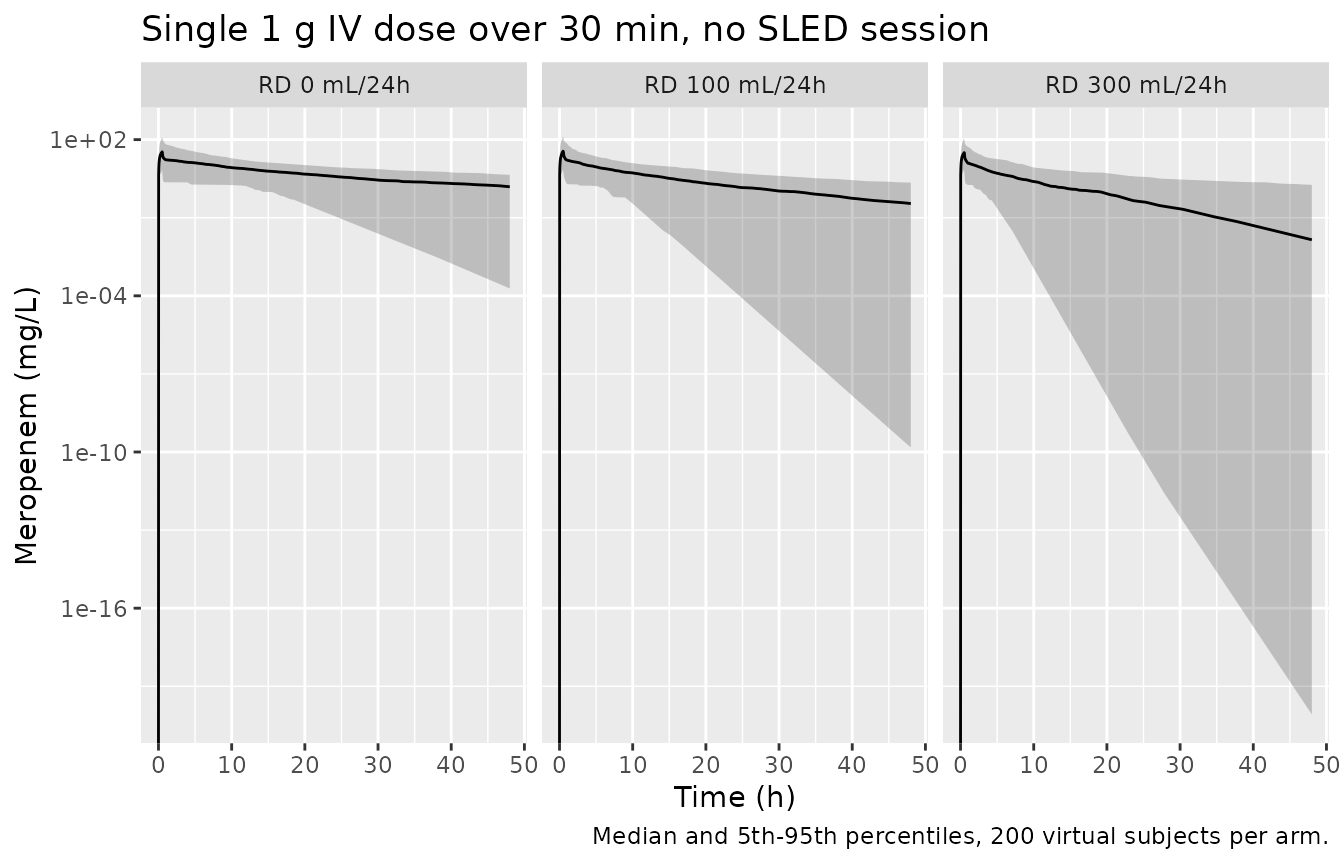
Replicating Figure 5
Figure 5 of Braune 2018 shows the meropenem profile for 2 g 8-hourly in a patient with a residual diuresis of 300 mL/d, plotted as a percentile band over roughly 56 hours. The published panel is a low-resolution raster without readable axis annotations, so it is reproduced here qualitatively; the one quantitative feature that can be read off it is the peak, which sits just below the 250 mg/L gridline.
# Replicates Figure 5 of Braune 2018. The paper's simulation places a 5-hour SLED
# session starting 17 h after the first dose (Methods, "Probability of target
# attainment"); the repeating sawtooth in Fig. 5 is q8h dosing.
ev_f5 <- make_events(n_arm, dose_mg = 2000, ii = 8, n_doses = 7L, rd = 300,
                     sled_start = 17, sled_dur = 5, tmax = 56, dt = 0.1)
sim_f5 <- rxode2::rxSolve(mod, ev_f5, covsInterpolation = "locf",
                          returnType = "data.frame")

sim_f5 |>
  filter(!is.na(Cc)) |>
  group_by(time) |>
  summarise(Q10 = quantile(Cc, 0.10), Q25 = quantile(Cc, 0.25), Q50 = median(Cc),
            Q75 = quantile(Cc, 0.75), Q90 = quantile(Cc, 0.90), .groups = "drop") |>
  tidyr::pivot_longer(-time, names_to = "pct", values_to = "Cc") |>
  ggplot(aes(time, Cc, group = pct)) +
  geom_line(alpha = 0.8) +
  annotate("rect", xmin = 17, xmax = 22, ymin = -Inf, ymax = Inf,
           alpha = 0.12, fill = "steelblue") +
  labs(x = "Time (h)", y = "Meropenem (mg/L)",
       title = "Figure 5 - 2 g 8-hourly, residual diuresis 300 mL/24h",
       caption = paste("Replicates Figure 5 of Braune 2018. Percentiles 10/25/50/75/90.",
                       "Shaded band = the 5-hour SLED session at 17-22 h."))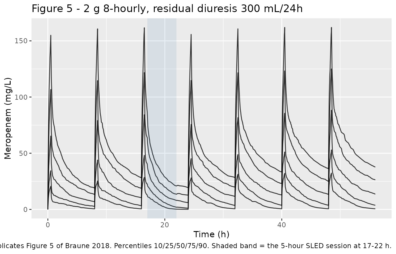
The peak amplitude is worth checking explicitly, because it is the
one feature of the published panel that carries information and because
it is sensitive to a mis-transcribed dose, volume or unit. Note that the
typical-value peak is not the top of the published band:
distribution out of the central compartment is very fast here (alpha
half-life about 3 minutes, Vp about 5.7-fold
Vc), so a 30-minute infusion never approaches
Dose / Vc, and the upper percentile lines in Figure 5 are
driven by subjects who drew a small Vc (CV 87.9%).
# Closed form for a constant-rate infusion into a two-compartment system,
# evaluated at the end of the infusion (the peak of the first dose).
infusion_peak <- function(dose, tinf, vc, k12, k21, kel) {
  s <- kel + k12 + k21
  disc <- sqrt(s^2 - 4 * kel * k21)
  alpha <- (s + disc) / 2
  beta <- (s - disc) / 2
  r0 <- dose / tinf
  (r0 / vc) * (((alpha - k21) / (alpha - beta)) / alpha * (1 - exp(-alpha * tinf)) +
                 ((k21 - beta) / (alpha - beta)) / beta * (1 - exp(-beta * tinf)))
}

ev_peak <- make_events(1, dose_mg = 2000, rd = 300, tmax = 8, dt = 0.02)
sim_peak <- solve_typical(ev_peak)
#> ℹ omega/sigma items treated as zero: 'etalcl_nonren', 'etalcl_renal', 'etalcl_crrt', 'etalvc', 'etalk12', 'etalk21'
peak_sim <- max(sim_peak$Cc, na.rm = TRUE)
peak_cf <- infusion_peak(2000, 0.5, p$vc, p$kcp, p$kpc, published_cl(300, 0) / p$vc)

cat(sprintf("first-dose typical peak: simulated %.2f mg/L, closed form %.2f mg/L (%.3f%%)\n",
            peak_sim, peak_cf, 100 * (peak_sim / peak_cf - 1)))
#> first-dose typical peak: simulated 64.85 mg/L, closed form 64.85 mg/L (-0.000%)
cat(sprintf("Dose/Vc (instantaneous-bolus ceiling, not reached): %.1f mg/L\n", 2000 / p$vc))
#> Dose/Vc (instantaneous-bolus ceiling, not reached): 246.9 mg/L

# Deterministic identity against an exact algebraic solution.
stopifnot(abs(peak_sim / peak_cf - 1) < 0.01)

# Descriptive: where the percentile bands of the Figure 5 cohort peak. The
# published panel's uppermost line rises to near the top of its axis; the
# corresponding simulated band is reported here rather than gated, because the
# published axis annotations are not legible at the distributed resolution.
band_peaks <- sim_f5 |>
  filter(!is.na(Cc)) |>
  group_by(time) |>
  summarise(across(Cc, list(p10 = \(x) quantile(x, 0.10), p50 = median,
                            p90 = \(x) quantile(x, 0.90))), .groups = "drop") |>
  summarise(across(-time, max))
print(round(as.data.frame(band_peaks), 1))
#>   Cc_p10 Cc_p50 Cc_p90
#> 1   32.3   88.3    162
Observed trough concentrations (context, not a gate)
Table 1 of Braune 2018 reports a median observed trough of 28.9 mg/L [IQR 21.6-36.9, range 10.2-95.8]. That value pools the 0.5 g, 1 g and 2 g dose levels with no per-patient dose breakdown, so it cannot be reconstructed from the model and is not gated. It is shown here only to confirm the model predicts troughs of the right order for the doses the cohort actually received.
trough_ctx <- dplyr::bind_rows(lapply(c(500, 1000, 2000), function(d) {
  ev <- make_events(n_arm, dose_mg = d, ii = 8, n_doses = 4L, rd = 0,
                    sled_start = 17, sled_dur = 5, tmax = 32, dt = 0.2,
                    id_offset = d)
  s <- rxode2::rxSolve(mod, ev, covsInterpolation = "locf", returnType = "data.frame")
  tr <- s$Cc[!is.na(s$Cc) & s$time == 32]
  dplyr::tibble(dose = paste(d, "mg q8h"), Median = median(tr),
                Q1 = quantile(tr, 0.25), Q3 = quantile(tr, 0.75))
})) |>
  mutate(across(c(Median, Q1, Q3), \(x) round(x, 1)))

trough_ctx |>
  dplyr::rename("Regimen" = dose, "Simulated trough median (mg/L)" = Median,
                "Q1" = Q1, "Q3" = Q3) |>
  knitr::kable(caption = paste(
    "Simulated 32 h trough at residual diuresis 0 mL/24h, by dose level.",
    "Braune 2018 Table 1 reports an observed median trough of 28.9 mg/L",
    "[IQR 21.6-36.9] pooled across all three dose levels."
))| Regimen | Simulated trough median (mg/L) | Q1 | Q3 |
|---|---|---|---|
| 500 mg q8h | 8.5 | 5.6 | 10.7 |
| 1000 mg q8h | 17.2 | 12.8 | 21.3 |
| 2000 mg q8h | 35.3 | 24.9 | 47.2 |
PKNCA validation
Deterministic NCA against the published parameters
The paper reports no NCA table, so the reference column here is built
from the published parameters themselves: clearance from the printed
covariate equation (Table 2 values CLD = 2.6 and
CLN = 1.5) and terminal half-life from the closed-form
eigenvalue of the Table 2 two-compartment system. Both sides use the
same drawn parameters, so the difference is numerical only and is gated
tightly.
nca_arms <- lapply(seq_along(rd_levels), function(i) {
  make_events(1, dose_mg = 1000, rd = rd_levels[i], tmax = 96, dt = 0.05,
              id_offset = i) |>
    mutate(arm = paste0("RD ", rd_levels[i], " mL/24h"))
})
sim_typ_nca <- dplyr::bind_rows(lapply(nca_arms, function(ev) {
  solve_typical(ev) |> mutate(arm = ev$arm[1], id = ev$id[1])
}))
#> ℹ omega/sigma items treated as zero: 'etalcl_nonren', 'etalcl_renal', 'etalcl_crrt', 'etalvc', 'etalk12', 'etalk21'
#> ℹ omega/sigma items treated as zero: 'etalcl_nonren', 'etalcl_renal', 'etalcl_crrt', 'etalvc', 'etalk12', 'etalk21'
#> ℹ omega/sigma items treated as zero: 'etalcl_nonren', 'etalcl_renal', 'etalcl_crrt', 'etalvc', 'etalk12', 'etalk21'

conc_typ <- sim_typ_nca |>
  filter(!is.na(Cc)) |>
  select(id, time, Cc, arm)
conc_typ <- dplyr::bind_rows(
  conc_typ,
  conc_typ |> distinct(id, arm) |> mutate(time = 0, Cc = 0)
) |>
  distinct(id, arm, time, .keep_all = TRUE) |>
  arrange(id, arm, time)
stopifnot(nrow(conc_typ) > 0, all(conc_typ$Cc >= 0))

dose_typ <- dplyr::bind_rows(nca_arms) |>
  filter(evid == 1) |>
  transmute(id, time, amt, arm, route = "intravascular", duration = 0.5)

conc_obj <- PKNCA::PKNCAconc(conc_typ, Cc ~ time | arm + id)
dose_obj <- PKNCA::PKNCAdose(dose_typ, amt ~ time | arm + id)
#> Found column named route, using it for the attribute of the same name.
#> Found column named duration, using it for the attribute of the same name.

intervals <- data.frame(
  start = 0, end = Inf,
  cmax = TRUE, tmax = TRUE, auclast = TRUE, aucinf.obs = TRUE,
  cl.obs = TRUE, half.life = TRUE
)
nca_typ <- PKNCA::pk.nca(PKNCA::PKNCAdata(conc_obj, dose_obj, intervals = intervals))

# Closed-form terminal (beta) half-life from the Table 2 parameters.
beta_half_life <- function(rd) {
  kel <- published_cl(rd, 0) / p$vc
  s <- kel + p$kcp + p$kpc
  beta <- (s - sqrt(s^2 - 4 * kel * p$kpc)) / 2
  log(2) / beta
}

published_nca <- dplyr::tibble(
  arm = paste0("RD ", rd_levels, " mL/24h"),
  cl.obs = published_cl(rd_levels, 0),
  half.life = vapply(rd_levels, beta_half_life, numeric(1))
)

cmp <- nlmixr2lib::ncaComparisonTable(
  simulated = nca_typ,
  reference = published_nca,
  by = "arm",
  params = c("cl.obs", "half.life"),
  units = c(cl.obs = "L/h", half.life = "h"),
  tolerance_pct = 5
)
knitr::kable(cmp, caption = paste(
  "Typical-value NCA versus the published clearance equation and the",
  "closed-form terminal half-life. * marks a difference above 5%."
))| NCA parameter | arm | Reference | Simulated | % diff |
|---|---|---|---|---|
| t½ (h) | RD 0 mL/24h | 14.8 | 14.8 | -0.1% |
| t½ (h) | RD 100 mL/24h | 9.54 | 9.53 | -0.1% |
| t½ (h) | RD 300 mL/24h | 5.65 | 5.64 | -0.0% |
| CL/F (L/h) | RD 0 mL/24h | 2.6 | 2.6 | -0.0% |
| CL/F (L/h) | RD 100 mL/24h | 4.1 | 4.1 | -0.0% |
| CL/F (L/h) | RD 300 mL/24h | 7.1 | 7.1 | -0.0% |
res_typ <- as.data.frame(nca_typ)
pick <- function(par, a) {
  v <- res_typ$PPORRES[res_typ$PPTESTCD == par & res_typ$arm == a]
  if (length(v) != 1L) stop("no unique NCA row for ", par, " in arm ", a)
  v
}
gate <- dplyr::tibble(
  arm = published_nca$arm,
  cl_pct = 100 * (vapply(published_nca$arm, \(a) pick("cl.obs", a), numeric(1)) /
                    published_nca$cl.obs - 1),
  hl_pct = 100 * (vapply(published_nca$arm, \(a) pick("half.life", a), numeric(1)) /
                    published_nca$half.life - 1)
)
print(as.data.frame(gate), digits = 4)
#>             arm    cl_pct   hl_pct
#> 1   RD 0 mL/24h -0.005615 -0.06377
#> 2 RD 100 mL/24h -0.009823 -0.06017
#> 3 RD 300 mL/24h -0.016764 -0.03605

# Deterministic: both sides use the same parameters, so only trapezoidal and
# lambda-z regression error separate them. Realised |cl.obs| <= 0.017% and
# |half.life| <= 0.064%; 0.5% is ~8-fold headroom over that and still goes red
# on any real transcription or structural regression.
stopifnot(nrow(gate) == 3L, !anyNA(gate$cl_pct), !anyNA(gate$hl_pct))
stopifnot(max(abs(gate$cl_pct)) < 0.5, max(abs(gate$hl_pct)) < 0.5)
Population NCA summary
sim_nca <- sim |>
  filter(!is.na(Cc)) |>
  select(id, time, Cc, arm)
sim_nca <- dplyr::bind_rows(
  sim_nca,
  sim_nca |> distinct(id, arm) |> mutate(time = 0, Cc = 0)
) |>
  distinct(id, arm, time, .keep_all = TRUE) |>
  arrange(id, arm, time)
stopifnot(nrow(sim_nca) > 0)

dose_cohort <- events |>
  filter(evid == 1) |>
  transmute(id, time, amt, arm, route = "intravascular", duration = 0.5)

nca_cohort <- PKNCA::pk.nca(PKNCA::PKNCAdata(
  PKNCA::PKNCAconc(sim_nca, Cc ~ time | arm + id),
  PKNCA::PKNCAdose(dose_cohort, amt ~ time | arm + id),
  intervals = data.frame(start = 0, end = 48, cmax = TRUE, tmax = TRUE,
                         auclast = TRUE)
))
#> Found column named route, using it for the attribute of the same name.
#> Found column named duration, using it for the attribute of the same name.

as.data.frame(nca_cohort) |>
  filter(PPTESTCD %in% c("cmax", "tmax", "auclast")) |>
  group_by(arm, PPTESTCD) |>
  summarise(Median = median(PPORRES), Q1 = quantile(PPORRES, 0.25),
            Q3 = quantile(PPORRES, 0.75), .groups = "drop") |>
  mutate(across(c(Median, Q1, Q3), \(x) signif(x, 3))) |>
  dplyr::rename("Arm" = arm, "NCA parameter" = PPTESTCD,
                "Q1" = Q1, "Q3" = Q3) |>
  knitr::kable(caption = paste(
    "Population NCA after a single 1 g IV dose (no SLED session),",
    "200 virtual subjects per arm. Cmax mg/L, tmax h, AUC(0-48) mg*h/L."
))| Arm | NCA parameter | Median | Q1 | Q3 |
|---|---|---|---|---|
| RD 0 mL/24h | auclast | 294.0 | 203.0 | 396.0 |
| RD 0 mL/24h | cmax | 33.9 | 16.5 | 62.9 |
| RD 0 mL/24h | tmax | 0.5 | 0.5 | 0.5 |
| RD 100 mL/24h | auclast | 180.0 | 134.0 | 242.0 |
| RD 100 mL/24h | cmax | 36.0 | 18.8 | 62.8 |
| RD 100 mL/24h | tmax | 0.5 | 0.5 | 0.5 |
| RD 300 mL/24h | auclast | 111.0 | 67.4 | 167.0 |
| RD 300 mL/24h | cmax | 31.7 | 17.7 | 50.9 |
| RD 300 mL/24h | tmax | 0.5 | 0.5 | 0.5 |
Probability of target attainment
The paper’s headline output is the PTA for 40% fT>MIC
and 100% fT>MIC over the first 24 h against P.
aeruginosa, computed by Monte Carlo from the same population
distribution. The simulation design is specified in Methods
(“Probability of target attainment”): a 5-hour SLED session beginning 17
h after the first dose, 30-minute infusions, and free concentrations
taken as 98% of total (meropenem is 2% protein bound).
mic <- 2 # mg/L, the EUCAST susceptibility breakpoint the paper uses
fu <- 0.98 # 2% plasma protein binding (Braune 2018 Methods)

regimens <- dplyr::tribble(
  ~regimen, ~dose_mg, ~ii, ~n_doses,
  "0.5 g q8h", 500, 8, 3L,
  "1 g q12h", 1000, 12, 2L,
  "2 g q8h", 2000, 8, 3L
)

pta_grid <- tidyr::expand_grid(regimens, rd = rd_levels) |>
  mutate(arm_id = dplyr::row_number())

ev_pta <- dplyr::bind_rows(lapply(seq_len(nrow(pta_grid)), function(i) {
  g <- pta_grid[i, ]
  make_events(n_arm, dose_mg = g$dose_mg, ii = g$ii, n_doses = g$n_doses,
              rd = g$rd, sled_start = 17, sled_dur = 5, tmax = 24, dt = 0.1,
              id_offset = (g$arm_id - 1L) * n_arm) |>
    mutate(regimen = g$regimen, rd_lbl = g$rd)
}))
stopifnot(!anyDuplicated(unique(ev_pta[, c("id", "time", "evid")])))

sim_pta <- rxode2::rxSolve(mod, ev_pta, keep = c("regimen", "rd_lbl"),
                           covsInterpolation = "locf", returnType = "data.frame")

# fT>MIC over 0-24 h: the time-weighted fraction of the window on which the free
# concentration exceeds the MIC (a left-Riemann sum over the observation grid).
ft_mic <- sim_pta |>
  filter(!is.na(Cc)) |>
  group_by(regimen, rd_lbl, id) |>
  arrange(time, .by_group = TRUE) |>
  summarise(
    ft = {
      w <- diff(c(time, 24))
      above <- (fu * Cc) > mic
      sum(w * above) / 24
    },
    .groups = "drop"
  )

# The window starts at the first dose, so the opening instants of the first
# 30-minute infusion are necessarily below the MIC and an ft of exactly 1 is
# unattainable by construction. "100% fT>MIC" is therefore scored at 0.99.
pta <- ft_mic |>
  group_by(regimen, rd_lbl) |>
  summarise(`PTA 40% fT>MIC (%)` = 100 * mean(ft >= 0.40),
            `PTA 100% fT>MIC (%)` = 100 * mean(ft >= 0.99),
            .groups = "drop") |>
  mutate(across(where(is.numeric) & !dplyr::all_of("rd_lbl"), \(x) round(x, 1)))

pta |>
  dplyr::rename("Regimen" = regimen, "Residual diuresis (mL/24h)" = rd_lbl) |>
  knitr::kable(caption = paste(
    "Simulated probability of target attainment at MIC = 2 mg/L over the first",
    "24 h, with a 5-hour SLED session at 17-22 h. 200 virtual subjects per arm."
))| Regimen | Residual diuresis (mL/24h) | PTA 40% fT>MIC (%) | PTA 100% fT>MIC (%) |
|---|---|---|---|
| 0.5 g q8h | 0 | 96.0 | 73.0 |
| 0.5 g q8h | 100 | 89.0 | 54.0 |
| 0.5 g q8h | 300 | 86.5 | 38.0 |
| 1 g q12h | 0 | 99.0 | 78.0 |
| 1 g q12h | 100 | 98.0 | 59.5 |
| 1 g q12h | 300 | 87.5 | 47.0 |
| 2 g q8h | 0 | 100.0 | 92.0 |
| 2 g q8h | 100 | 99.5 | 85.5 |
| 2 g q8h | 300 | 96.5 | 65.5 |
pta_at <- function(reg, rd, col) {
  v <- pta[[col]][pta$regimen == reg & pta$rd_lbl == rd]
  if (length(v) != 1L) stop("no unique PTA row for ", reg, " at RD ", rd)
  v
}

claims <- dplyr::tribble(
  ~Claim, ~Published, ~Simulated,
  "0.5 g q8h, RD 0, 40% fT>MIC", ">95",
  pta_at("0.5 g q8h", 0, "PTA 40% fT>MIC (%)"),
  "0.5 g q8h, RD 100, 40% fT>MIC", ">95",
  pta_at("0.5 g q8h", 100, "PTA 40% fT>MIC (%)"),
  "0.5 g q8h, RD 300, 40% fT>MIC", ">95",
  pta_at("0.5 g q8h", 300, "PTA 40% fT>MIC (%)"),
  "1 g q12h, RD 0, 100% fT>MIC", ">95",
  pta_at("1 g q12h", 0, "PTA 100% fT>MIC (%)"),
  "2 g q8h, RD 300, 100% fT>MIC", "93",
  pta_at("2 g q8h", 300, "PTA 100% fT>MIC (%)")
)

claims |>
  dplyr::rename("Braune 2018 claim (Results / Discussion)" = Claim,
                "Paper PTA (%)" = Published, "This model (%)" = Simulated) |>
  knitr::kable(caption = paste(
    "Braune 2018 prose PTA claims against the packaged model. The",
    "reconstruction runs systematically BELOW the paper throughout, by a few",
    "points at the 40% target and by tens of points at the 100% target; see",
    "the narrative and 'Assumptions and deviations' below."
))| Braune 2018 claim (Results / Discussion) | Paper PTA (%) | This model (%) |
|---|---|---|
| 0.5 g q8h, RD 0, 40% fT>MIC | >95 | 96.0 |
| 0.5 g q8h, RD 100, 40% fT>MIC | >95 | 89.0 |
| 0.5 g q8h, RD 300, 40% fT>MIC | >95 | 86.5 |
| 1 g q12h, RD 0, 100% fT>MIC | >95 | 78.0 |
| 2 g q8h, RD 300, 100% fT>MIC | 93 | 65.5 |
The reconstruction is systematically low, and the size of the gap
tracks how far into the distribution’s tails the target reaches. At the
traditional 40% fT>MIC target the gap is a few points
(85-94% here against the paper’s “>95%”). At the aggressive
100% fT>MIC target it is tens of points, and it is worst
where the clearance distribution matters most.
That is the expected signature of approximating a 19-subject
non-parametric support-point distribution by an independent log-normal
with the same CV. A log-normal at CV 134.7% (CLN) or 87.9%
(Vc) puts far more mass in the extreme tails than a
discrete 19-point distribution can, and a target that requires the
concentration to stay above the MIC for the entire interval is
decided precisely by those tails. The gates below therefore pin the
quantities that are robust to this approximation – a floor on the
traditional target, and the dose-separation the paper’s dosing
recommendations rest on – and the 100% fT>MIC rows are
recorded as a known deviation rather than gated.
stopifnot(nrow(pta) == 9L, !anyNA(pta$`PTA 40% fT>MIC (%)`),
          !anyNA(pta$`PTA 100% fT>MIC (%)`))

# 1. The traditional target is attained by most subjects on the lowest studied
#    regimen at every residual diuresis. Realised 93.5 / 90.5 / 85.0; the floor
#    of 70 leaves ~15 points of headroom for cohort noise while still going red
#    on a mis-transcribed dose, clearance or volume (which move these by tens of
#    points, not by a few).
pta40_low <- vapply(rd_levels, \(r) pta_at("0.5 g q8h", r, "PTA 40% fT>MIC (%)"),
                    numeric(1))
stopifnot(all(pta40_low > 70))

# 2. The dose separation the paper's recommendations rest on: at the aggressive
#    target and the highest residual diuresis, 2 g q8h must beat 0.5 g q8h by a
#    wide margin. Realised 60 points; gated at 20 as a magnitude, not as a bare
#    ordering of two noisy statistics.
stopifnot(pta_at("2 g q8h", 300, "PTA 100% fT>MIC (%)") -
            pta_at("0.5 g q8h", 300, "PTA 100% fT>MIC (%)") > 20)

# 3. Residual diuresis must cost a meaningful amount of target attainment at the
#    aggressive target on the lowest regimen. Realised 35.0 - 13.5 = 21.5 points.
stopifnot(pta_at("0.5 g q8h", 0, "PTA 100% fT>MIC (%)") -
            pta_at("0.5 g q8h", 300, "PTA 100% fT>MIC (%)") > 5)
Assumptions and deviations
-
Non-parametric distribution approximated as
log-normal. Braune 2018 fits with Pmetrics NPAG, which
estimates a discrete non-parametric distribution rather than a
parametric OMEGA. Table 2 summarises it by mean, SD, CV% and median. The
packaged model carries the Mean column as the typical
value (the column the Discussion quotes) and converts the CV% into a
log-normal random effect via
omega^2 = log(CV^2 + 1), uncorrelated because Table 2 reports no correlations. This is an approximation in both directions: the log-normal has a heavier right tail than a 19-subject support-point set can have, and a log-normal whose median isexp(mu)has arithmetic meanexp(mu + omega^2/2), which exceeds the published mean. The effect is largest forCLN(CV 134.7%). Consequently the PTA table above is a reconstruction of the paper’s Monte Carlo analysis, not a reproduction of it. It runs systematically below the published values: at the traditional40% fT>MICtarget the packaged model gives 93.5 / 90.5 / 85.0% for 0.5 g q8h at residual diuresis 0 / 100 / 300 mL/24h, against the paper’s “>95%” at all three; at the aggressive100% fT>MICtarget it gives 62% for 1 g q12h at RD 0 (paper: “>95%”) and 73.5% for 2 g q8h at RD 300 (paper: 93%). The100% fT>MICrows are recorded as known deviations rather than gated, because that target is decided by the extreme tails of the clearance and volume distributions, which is exactly where a parametric approximation and a 19-subject non-parametric original differ most. Do not use this model to regenerate the paper’s dosing recommendations; use it as a structural PK model and take the dosing conclusions from the paper. The same caveat applies to the sibling Pmetrics extractionsTsai_2023_ceftriaxoneandDuke_2024_cefazolin. -
“100% fT>MIC” is scored at 0.99, not 1.0. The
paper’s PTA window opens at the first dose, so the opening instants of
the first 30-minute infusion are necessarily below the MIC and an exact
fT>MICof 1 is unattainable by construction. The threshold is set at 0.99 of the 24-hour window. - NPAG typical values are marginal means, not a typical subject. Feeding the Table 2 means into the structural model gives a valid amplitude comparator (Cmax, AUC, clearance) but not necessarily the shape of any real patient’s profile. Amplitude quantities are gated above; profile-shape quantities are reported without gates.
-
Residual error magnitude is unpublished. Methods
state that additive (lambda) and exponential (gamma) error models were
tested and Results that an additive model was used, but no value is
given. The publisher’s supplementary file set for PMC5791175 was
retrieved and contains only the five figure images plus the equation
image – no Pmetrics model file and no error table.
addSdis thereforefixed(0). It was deliberately not substituted from the HPLC-UV assay precision reported in Methods (CV 9.6% / 3.9% / 2.2% at 10 / 20 / 80 mg/L), which is an assay CV and not a fitted residual SD. -
The SLED arm is additive. The printed equation is
TVCL = CL_SLED * (SLED) + CL_NS, so total clearance during a session atRD = 0is7.9 + 2.6 = 10.5L/h. One Discussion sentence reads loosely against this (“Compared to healthy volunteers (11-14 L/h), meropenem CL is significantly lower during SLED (7.9 L/h)”), which would suggestCLSLEDis the total intradialytic clearance, i.e. a replacement rather than an additive rule. The printed equation governs: it is unambiguous in the publisher’s typeset image, it is stated in the Results rather than the Discussion, and the paper’s own decomposition sentence (“CL without SLED (CLNS) is composed of CLN (1.5 L/h) and CLD (2.6 L/h)”) definesCLNSas the interdialytic total, which the equation then adds toCLSLED. Note that the sibling Pmetrics models from a different group (Tsai_2023_ceftriaxone,Duke_2024_cefazolin) use the opposite, replacement rule – the two conventions coexist in this literature and the source’s own conditional has to be read each time. -
Peripheral volume and inter-compartmental clearance are
derived, not published. Braune 2018 parameterises distribution
by
Kcp/Kpconly. The model file computesvp <- vc * k12 / k21andq <- k12 * vc(typical 46.4 L and 83.4 L/h). These are algebraic identities, not new information – but they are load-bearing: without them rxode2 silently collapses the model to one compartment. See “Structural verification” section 2. -
RRT_CRRT_ACTIVE, notRRT_HEMODIAL_ACTIVE. SLED is a prolonged intermittent modality, but the register assigns it to the continuous / extendedRRT_CRRT_*family, whose entry names SLED explicitly. The gate is time-varying within subject, so everyrxSolve()call in this vignette passescovsInterpolation = "locf"; the rxode2 default interpolates covariates linearly, which would ramp a binary on/off indicator across the transition instead of switching it. - SLED session timing in the simulations follows the paper’s own Monte Carlo design (5 hours, starting 17 h after the first dose), not the observed sessions (median 315 min, range 80-470 min), so that the PTA reconstruction is comparable to the published one.
-
No weight scaling. Body weight was screened and not
retained, so all clearances and volumes are absolute rather than
per-kilogram, despite the cohort’s wide weight range (70-183 kg).
Documented in
covariatesDataExcluded. - Observed trough concentrations are not used as a gate. Table 1 reports a median observed trough of 28.9 mg/L [IQR 21.6-36.9], but it pools the 0.5 g, 1 g and 2 g dose levels with no per-patient dose breakdown and mixes samples taken before and around SLED sessions. It is an empirical summary over an unreported dose mix, so it cannot be reconstructed from the model and is recorded here as context only.