Oral paclitaxel boosted with ritonavir, and thrombospondin-1 (van Eijk 2022)
Source:vignettes/articles/vanEijk_2022_paclitaxel.Rmd
vanEijk_2022_paclitaxel.RmdModel and source
- Citation: van Eijk M, Yu H, Sawicki E, de Weger VA, Nuijen B, Dorlo TPC, Beijnen JH, Huitema ADR. Development of a population pharmacokinetic/pharmacodynamic model for various oral paclitaxel formulations co-administered with ritonavir and thrombospondin-1 based on data from early phase clinical studies. Cancer Chemother Pharmacol. 2022;90(1):71-82. doi:10.1007/s00280-022-04445-z. Embedded ritonavir PK model (structure and all ritonavir parameter values) from Yu H, Janssen JM, Sawicki E, van Hasselt JGC, de Weger VA, Nuijen B, Schellens JHM, Beijnen JH, Huitema ADR. A Population Pharmacokinetic Model of Oral Docetaxel Coadministered With Ritonavir to Support Early Clinical Development. J Clin Pharmacol. 2020;60(3):340-350. doi:10.1002/jcph.1532 (van Eijk 2022 reference [29]; Table 2 and Equation 3).
- Description: Semi-physiological population PK/PD model for oral paclitaxel (drinking solution, ModraPac capsule and ModraPac tablet) co-administered with oral ritonavir in adult cancer patients: Weibull-type gut absorption into a 1 L well-stirred liver compartment whose intrinsic clearance is inhibited by the ritonavir plasma concentration (Imax model), two-compartment systemic disposition, an embedded two-compartment ritonavir PK model with inverse Gaussian absorption (Yu 2020), and a thrombospondin-1 (TSP-1) turnover model whose formation rate is stimulated by paclitaxel (Emax = 1)
- Article: https://doi.org/10.1007/s00280-022-04445-z (open access)
- Embedded ritonavir model: Yu et al. 2020, https://doi.org/10.1002/jcph.1532
van Eijk et al. pooled three early-phase studies of oral paclitaxel given with the CYP3A4 inhibitor ritonavir. Three oral formulations were studied: the intravenous formulation taken as a drinking solution, and the ModraPac capsule and ModraPac tablet (amorphous solid dispersions). The PK model has four paclitaxel compartments: gut, a 1 L well-stirred liver, central and peripheral. Gut absorption is time-varying (a Weibull function). The intrinsic clearance in the liver is reduced by the ritonavir plasma concentration through an Imax model, and ritonavir itself follows the previously published Yu 2020 model. A turnover model for the anti-angiogenic marker thrombospondin-1 (TSP-1) has its formation rate stimulated by paclitaxel.
Population
The PK analysis pooled 58 adult cancer patients from three studies:
- Study 1: a single 100 mg dose of the paclitaxel drinking solution, with 100 or 200 mg ritonavir 30 min earlier (17 patients).
- Study 2: a randomised crossover of the drinking solution and the ModraPac capsule, 30 mg once weekly with 100 mg ritonavir (4 patients).
- Study 3: a phase I low-dose metronomic (LDM) dose escalation (37 patients). Capsule (5-40 mg/day) or tablet (40-60 mg/day) was taken twice daily, 7 h apart, each dose with ritonavir (200 mg/day in total).
TSP-1 was measured in 36 of the 37 Study 3 patients. The paper gives no demographic table, and the supplementary dose and sampling summary (Supplementary Table 1) is not part of the published supplementary file. The same information is available programmatically:
str(rxode2::rxode(readModelDb("vanEijk_2022_paclitaxel"))$population)
#> ℹ parameter labels from comments will be replaced by 'label()'
#> Warning: some etas defaulted to non-mu referenced, possible parsing error: etaiov_lfdepot_1, etaiov_lfdepot_2, etaiov_lmat_rtv_1, etaiov_lmat_rtv_2, etaiov_lcvabs_rtv_1, etaiov_lcvabs_rtv_2
#> as a work-around try putting the mu-referenced expression on a simple line
#> List of 8
#>  $ species      : chr "human"
#>  $ n_subjects   : num 58
#>  $ n_subjects_pd: num 36
#>  $ n_studies    : num 3
#>  $ disease_state: chr "adult cancer patients in three early-phase clinical studies of oral paclitaxel boosted with ritonavir"
#>  $ dose_range   : chr "Study 1: single 100 mg paclitaxel drinking solution with 100 or 200 mg ritonavir 30 min before (17 patients); S"| __truncated__
#>  $ regions      : chr "The Netherlands (Netherlands Cancer Institute)"
#>  $ notes        : chr "PK data from 58 patients in three studies (van Eijk 2022 Methods, 'Pharmacokinetic data'); TSP-1 PD data from 3"| __truncated__
Source trace
Every ini() value carries an in-file comment naming its
source. Ritonavir values come from Yu 2020, Table 2; van Eijk 2022
applied that model without re-estimating it.
| Equation / parameter | Value | Source location |
|---|---|---|
lra_dose1 = log(1/ALPHA) |
ALPHA 1.68 h | van Eijk Table 1, ALPHA 1st daily dose |
lra_dose2 = log(1/ALPHA) |
ALPHA 1.97 h | Table 1, ALPHA 2nd daily dose |
lgam1_sol / lgam1_asd
|
BETA 2.53 / 3.57 | Table 1, BETA drinking solution / tablet+capsule |
lfdepot |
1 (fixed) | Table 1, rF drinking solution 1 FIX |
e_form_tablet_fdepot /
e_form_capsule_fdepot
|
0.97 / 0.46 | Table 1, rF tablet / rF capsule |
e_dose2_fdepot |
0.59 | Table 1, rF 2nd/1st |
lclint |
746 L/h | Table 1, CL int0 |
limax |
570 L/h | Table 1, I max |
lki |
375 ng/mL | Table 1, KI |
qh, vh, fu
|
80 L/h, 1 L, 0.13 (fixed) | Methods, Pharmacokinetic model (refs 31-33) |
lvc, lq, lvp
|
128 L, 33.4 L/h, 375 L | Table 1 |
lrbase |
43.8 ng/mL/10^6 platelets | Table 2, E BASE |
lkout = log(1/Turnover) |
Turnover 233 h (fixed) | Table 2; Results (platelet survival 9.7 days) |
lec50 |
284 ng/mL | Table 2, EC50 |
lmat_rtv, lcvabs_rtv
|
8.45 h, 1.23 | Yu 2020 Table 2, MAT and CV |
lcl_rtv, lvc_rtv, lq_rtv,
lvp_rtv
|
7.72 L/h, 23 L, 3.99 L/h, 17.9 L | Yu 2020 Table 2 |
lfdepot2_rtv, lftab_rtv
|
2.25, 1.06 | Yu 2020 Table 2, F2nd/1st,rtv and Ftablet/capsule |
BSV etalra, etalclint,
etalvc, etalfdepot
|
35.1, 25.1, 53.8, 38.2 CV% | Table 1 |
BOV etaiov_lfdepot_1/2
|
45.8 CV% | Table 1 |
BSV etalrbase
|
28.2 CV% | Table 2 |
| ritonavir BSV and within-subject etas | 12.8-93.5 CV% | Yu 2020 Table 2 |
propSd, propSd_tsp1,
propSd_rtv
|
0.258, 0.138, 0.352 | Table 1, Table 2, Yu 2020 Table 2 |
clint <- clint0 - imax * Cc_rtv / (ki + Cc_rtv) |
Eq. 1 | |
eh <- clint * fu / (qh + clint * fu), F_H = 1 -
E_H |
Eqs. 2-3; Fig. 1 flows | |
Weibull ka(t)
|
Eq. 9 | |
| ritonavir inverse Gaussian input | Yu 2020 Eq. 3 | |
d/dt(tsp1) <- kin - kout * tsp1,
kin <- kin0 * (1 + Cc / (ec50 + Cc))
|
Eqs. 4-6 | |
BSV / BOV form P * exp(eta_BSV + eta_BOV)
|
Eq. 7 | |
| proportional residual error | Eq. 8 |
CV% values were converted to variances with omega^2 = log(1 + CV^2).
How to dose the model
mod <- readModelDb("vanEijk_2022_paclitaxel")
rxode2::rxode(mod)$state
#> ℹ parameter labels from comments will be replaced by 'label()'
#> Warning: some etas defaulted to non-mu referenced, possible parsing error: etaiov_lfdepot_1, etaiov_lfdepot_2, etaiov_lmat_rtv_1, etaiov_lmat_rtv_2, etaiov_lcvabs_rtv_1, etaiov_lcvabs_rtv_2
#> as a work-around try putting the mu-referenced expression on a simple line
#>  [1] "depot1"          "depot2"          "liver"           "central"
#>  [5] "peripheral1"     "depot1_rtv"      "depot2_rtv"      "central_rtv"
#> [9] "peripheral1_rtv" "tsp1"-
Paclitaxel: dose the first daily dose into
depot1and the second daily dose (7 h later) intodepot2. A once-daily, weekly or single dose goes intodepot1. -
Ritonavir: dose into
depot1_rtvanddepot2_rtvin the same way. -
Covariates: select the paclitaxel formulation with
FORM_TABLET/FORM_CAPSULE(both 0 means the drinking solution), and the ritonavir formulation withFORM_RTV_TABLET. -
Occasions:
OCC(1 or 2) selects the between-occasion etas, and 0 switches them off. -
Units: doses are in mg.
CcandCc_rtvare in ng/mL, andtsp1is in ng/mL/10^6 platelets. -
Observation rows: use
cmt = "tsp1". That is the model’s state endpoint, andCcandCc_rtvare returned on the same rows.
Two structural readings of the paper are needed to make the model simulate. The next sections test both against closed forms and against the paper’s own simulation results.
-
Absorption equation. Eq. 9 is printed as a rate
constant
ka(t) = (BETA/ALPHA) (t/ALPHA)^(BETA-1) exp(-(t/ALPHA)^BETA), withtthe time after the last dose. The model applies it literally, as a time-varying first-order rate constant on the gut amount. A single dose then leavesexp(-1)= 36.8% of the dose in the gut. That residue is absorbed when the next dose into the same compartment restarts the clock. - Ritonavir input. The inverse Gaussian density input (Yu 2020 Eq. 3) is applied as its hazard on a gut amount, which is exact for a single dose.
# One subject's twice-daily (7 h apart) regimen of paclitaxel + ritonavir,
# observation rows on the tsp1 state endpoint.
make_events <- function(ndays, pac_mg = 20, rtv_mg = 100, tab = 1L, cap = 0L,
                        grid = 0.05, id = 1L, occ = c(0L, 0L)) {
  k <- seq_len(ndays) - 1
  doses <- dplyr::bind_rows(
    data.frame(time = 24 * k, cmt = "depot1", amt = pac_mg, OCC = occ[1]),
    data.frame(time = 24 * k + 7, cmt = "depot2", amt = pac_mg, OCC = occ[2]),
    data.frame(time = 24 * k, cmt = "depot1_rtv", amt = rtv_mg, OCC = occ[1]),
    data.frame(time = 24 * k + 7, cmt = "depot2_rtv", amt = rtv_mg, OCC = occ[2])
  ) |>
    dplyr::mutate(evid = 1L)
  obs <- data.frame(time = seq(0, 24 * ndays, by = grid), cmt = "tsp1", amt = 0, evid = 0L)
  obs$OCC <- ifelse((obs$time %% 24) >= 7, occ[2], occ[1])
  dplyr::bind_rows(doses, obs) |>
    dplyr::arrange(time, dplyr::desc(evid)) |>
    dplyr::mutate(id = id, FORM_TABLET = tab, FORM_CAPSULE = cap, FORM_RTV_TABLET = 0L)
}
# Typical-value solve. zeroRe() is avoided on multi-endpoint models; omega = NA
# and sigma = NA give the same typical-value prediction.
solve_typical <- function(ev, ...) {
  rxode2::rxSolve(mod, ev, omega = NA, sigma = NA, useLinCmt = FALSE,
                  returnType = "data.frame", ...)
}
trap <- function(t, y) sum(diff(t) * (head(y, -1) + tail(y, -1)) / 2)
Closed-form checks of the two input functions
Paclitaxel (Eq. 9). With ka(t) equal to
the Weibull density, the gut amount after a single dose is
D * F * exp(-W(t)), where W is the Weibull
CDF. Without ritonavir the intrinsic clearance stays at
CLint0. A well-stirred liver compartment then gives
AUC0-inf = 1000 * A_abs / (fu * CLint0) ng*h/mL for an
absorbed amount A_abs in mg. Both identities are checked on
a 100 mg drinking-solution dose given with no ritonavir.
ev_cf <- dplyr::bind_rows(
  data.frame(time = 0, cmt = "depot1", amt = 100, evid = 1L),
  data.frame(time = c(seq(0, 24, by = 0.01), seq(24.5, 3000, by = 0.5)),
             cmt = "tsp1", amt = 0, evid = 0L)
) |>
  dplyr::mutate(id = 1L, FORM_TABLET = 0L, FORM_CAPSULE = 0L, FORM_RTV_TABLET = 0L, OCC = 0L)
cf <- solve_typical(ev_cf, rtol = 1e-10, atol = 1e-12)
#> ℹ parameter labels from comments will be replaced by 'label()'
#> Warning: some etas defaulted to non-mu referenced, possible parsing error: etaiov_lfdepot_1, etaiov_lfdepot_2, etaiov_lmat_rtv_1, etaiov_lmat_rtv_2, etaiov_lcvabs_rtv_1, etaiov_lcvabs_rtv_2
#> as a work-around try putting the mu-referenced expression on a simple line

alpha1 <- 1.68; beta_sol <- 2.53
gut_closed <- 100 * exp(-(1 - exp(-(cf$time / alpha1)^beta_sol)))
rel_gut <- max(abs(cf$depot1 / gut_closed - 1))
auc_sim <- trap(cf$time, cf$Cc)
auc_closed <- 1000 * 100 * (1 - exp(-1)) / (0.13 * 746)
c(max_rel_err_gut = rel_gut, auc_sim = auc_sim, auc_closed = auc_closed,
  rel_err_auc = auc_sim / auc_closed - 1)
#> max_rel_err_gut         auc_sim      auc_closed     rel_err_auc
#>    1.357029e-10    6.518103e+02    6.518051e+02    8.076944e-06
# Realised errors: 1.4e-10 on the gut amount (numerical ODE path at rtol
# 1e-10) and 8e-6 on the AUC (the trapezoid rule on the sampling grid plus
# the 3000 h truncation). A wrong rate-constant form or a wrong well-stirred
# relation moves these by tens of percent.
stopifnot(rel_gut < 1e-6, abs(auc_sim / auc_closed - 1) < 1e-3)
Ritonavir (Yu 2020 Eq. 3). After a single dose the
ritonavir gut amount equals
D * (1 - integral of the printed density). Here the
integral is taken numerically, straight from Eq. 3 as printed. That
makes it independent of the closed-form survivor the model uses for its
hazard.
ev_rt <- dplyr::bind_rows(
  data.frame(time = 0, cmt = "depot1_rtv", amt = 100, evid = 1L),
  data.frame(time = c(0.5, 1, 2, 4, 8, 12, 24, 48, 96), cmt = "tsp1", amt = 0, evid = 0L)
) |>
  dplyr::mutate(id = 1L, FORM_TABLET = 0L, FORM_CAPSULE = 0L, FORM_RTV_TABLET = 0L, OCC = 0L)
rt <- solve_typical(ev_rt, rtol = 1e-10, atol = 1e-12)
mat <- 8.45; cv <- 1.23
nin <- function(t) sqrt(mat / (2 * pi * cv^2 * t^3)) * exp(-(t - mat)^2 / (2 * cv^2 * mat * t))
remaining <- vapply(rt$time, function(t) 100 * (1 - integrate(nin, 0, t, rel.tol = 1e-10)$value), numeric(1))
rt_check <- data.frame(time = rt$time, model = rt$depot1_rtv, eq3 = remaining)
knitr::kable(rt_check, digits = 4, caption = "Ritonavir gut amount (mg) after a single 100 mg dose: model vs numerical integral of Yu 2020 Eq. 3.")| time | model | eq3 |
|---|---|---|
| 0.5 | 99.8418 | 99.8418 |
| 1.0 | 96.5993 | 96.5993 |
| 2.0 | 82.6247 | 82.6247 |
| 4.0 | 57.9947 | 57.9947 |
| 8.0 | 32.3049 | 32.3049 |
| 12.0 | 20.2061 | 20.2061 |
| 24.0 | 6.7418 | 6.7418 |
| 48.0 | 1.2649 | 1.2649 |
| 96.0 | 0.0846 | 0.0846 |
Reproduction of the paper’s simulations
The paper reports typical-value simulations at the recommended phase II dose (RP2D). That dose is 20 mg paclitaxel twice daily, 7 h apart, with ritonavir 100 mg twice daily:
- Results, “Simulations”, and Supplementary Figure S4: day-1 AUC0-24 for the capsule and the tablet, and Tmax in the first and second dose intervals.
- Results and Figure 4: a 3-week continuous tablet regimen with the steady-state Cmax, AUC0-504 and the cumulative time above 0.05 umol/L (42.7 ng/mL).
- Discussion: TSP-1 formation rate raised by 5.4% to 22.0% at steady state. With Eq. 6 this means steady-state paclitaxel concentrations of 16.2 to 80.1 ng/mL, since 284 * 0.054 / 0.946 = 16.2 and 284 * 0.22 / 0.78 = 80.1.
The paper does not say which ritonavir formulation these simulations
used, so the Yu 2020 reference capsule
(FORM_RTV_TABLET = 0) is used here.
d1_tab <- solve_typical(make_events(1, tab = 1L, cap = 0L))
d1_cap <- solve_typical(make_events(1, tab = 0L, cap = 1L))
w3_tab <- solve_typical(make_events(21, tab = 1L, cap = 0L))

tmax_in <- function(s, from, to) {
  w <- s[s$time >= from & s$time < to, ]
  w$time[which.max(w$Cc)] - from
}
ss <- w3_tab[w3_tab$time >= 480, ]
time_above <- sum(diff(w3_tab$time) * (head(w3_tab$Cc, -1) > 42.7))

repro <- tibble::tribble(
  ~quantity, ~published, ~model,
  "Day-1 AUC0-24, capsule (ug*h/L)", 131.4, trap(d1_cap$time, d1_cap$Cc),
  "Day-1 AUC0-24, tablet (ug*h/L)", 275.1, trap(d1_tab$time, d1_tab$Cc),
  "Tmax, first dose interval (h)", 2.1, tmax_in(d1_tab, 0, 7),
  "Tmax, second dose interval (h)", 2.4, tmax_in(d1_tab, 7, 24),
  "Steady-state Cmax, tablet (ng/mL)", 80.1, max(ss$Cc),
  "Steady-state Cmin implied by the 5.4% kin rise (ng/mL)", 284 * 0.054 / 0.946, min(ss$Cc),
  "AUC0-504, 3 weeks tablet (mg*h/L)", 16.0, trap(w3_tab$time, w3_tab$Cc) / 1000,
  "Cumulative time above 42.7 ng/mL over 3 weeks (h)", 115.6, time_above
) |>
  dplyr::mutate(pct_diff = 100 * (model / published - 1))
repro |>
  dplyr::rename("Quantity" = quantity, "Published" = published, "Model" = model,
                "Difference (%)" = pct_diff) |>
  knitr::kable(digits = c(0, 2, 2, 1),
caption = "Typical-value reproduction of the van Eijk 2022 simulations.")| Quantity | Published | Model | Difference (%) |
|---|---|---|---|
| Day-1 AUC0-24, capsule (ug*h/L) | 131.40 | 138.06 | 5.1 |
| Day-1 AUC0-24, tablet (ug*h/L) | 275.10 | 291.12 | 5.8 |
| Tmax, first dose interval (h) | 2.10 | 2.10 | 0.0 |
| Tmax, second dose interval (h) | 2.40 | 2.40 | 0.0 |
| Steady-state Cmax, tablet (ng/mL) | 80.10 | 81.44 | 1.7 |
| Steady-state Cmin implied by the 5.4% kin rise (ng/mL) | 16.21 | 16.66 | 2.8 |
| AUC0-504, 3 weeks tablet (mg*h/L) | 16.00 | 16.39 | 2.4 |
| Cumulative time above 42.7 ng/mL over 3 weeks (h) | 115.60 | 119.45 | 3.3 |
Every reported quantity is reproduced to within 6%, and both Tmax values match exactly. These are deterministic typical-value solves, so the bounds below are set close to the achieved accuracy. A mis-transcribed clearance, dose or absorption reading moves them by tens of percent. The day-1 AUC0-24 is 5-6% high. That is the largest structural difference and is discussed under “Assumptions and deviations”.
pd <- setNames(repro$pct_diff, repro$quantity)
stopifnot(
  abs(pd[["Day-1 AUC0-24, capsule (ug*h/L)"]]) < 8,
  abs(pd[["Day-1 AUC0-24, tablet (ug*h/L)"]]) < 8,
  abs(repro$model[3] - 2.1) <= 0.051,
  abs(repro$model[4] - 2.4) <= 0.051,
  abs(pd[["Steady-state Cmax, tablet (ng/mL)"]]) < 4,
  abs(pd[["AUC0-504, 3 weeks tablet (mg*h/L)"]]) < 5,
  abs(pd[[6]]) < 6,
  abs(pd[[8]]) < 8
)
ggplot(w3_tab, aes(time, Cc)) +
  geom_line(colour = "steelblue4") +
  geom_hline(yintercept = 42.7, linetype = "dashed") +
  labs(x = "Time (h)", y = "Paclitaxel (ng/mL)",
       title = "ModraPac tablet LDM, 3 weeks (typical values)")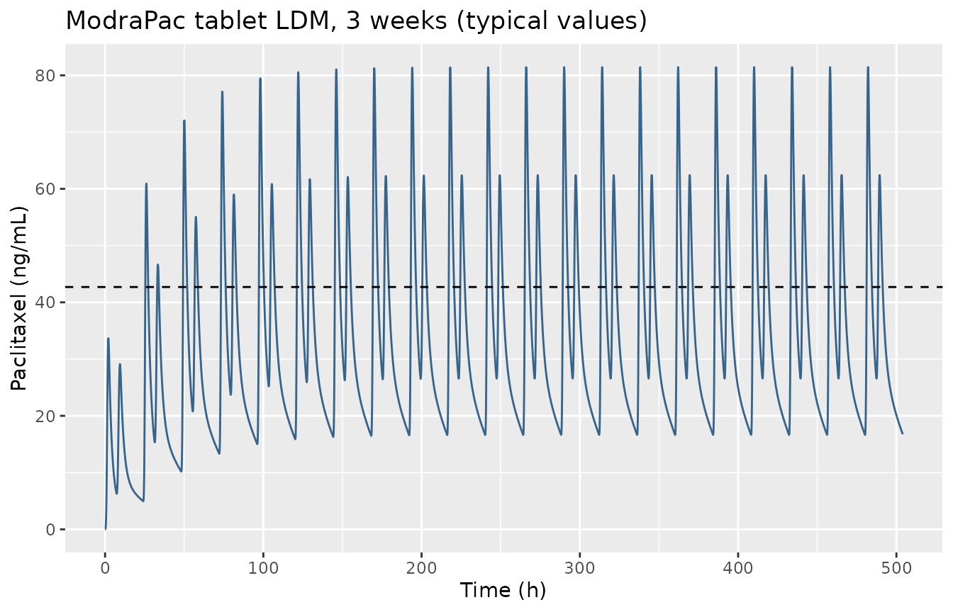
Replicates the ModraPac tablet curve of Figure 4 of van Eijk 2022: paclitaxel 20 mg twice daily (7 h apart) with ritonavir 100 mg twice daily, typical values, over 3 weeks. The dashed line is 42.7 ng/mL (0.05 umol/L).
dplyr::bind_rows(
  dplyr::mutate(d1_cap, formulation = "ModraPac capsule"),
  dplyr::mutate(d1_tab, formulation = "ModraPac tablet")
) |>
  ggplot(aes(time, Cc, colour = formulation)) +
  geom_line() +
  labs(x = "Time after first daily dose (h)", y = "Paclitaxel (ng/mL)", colour = NULL)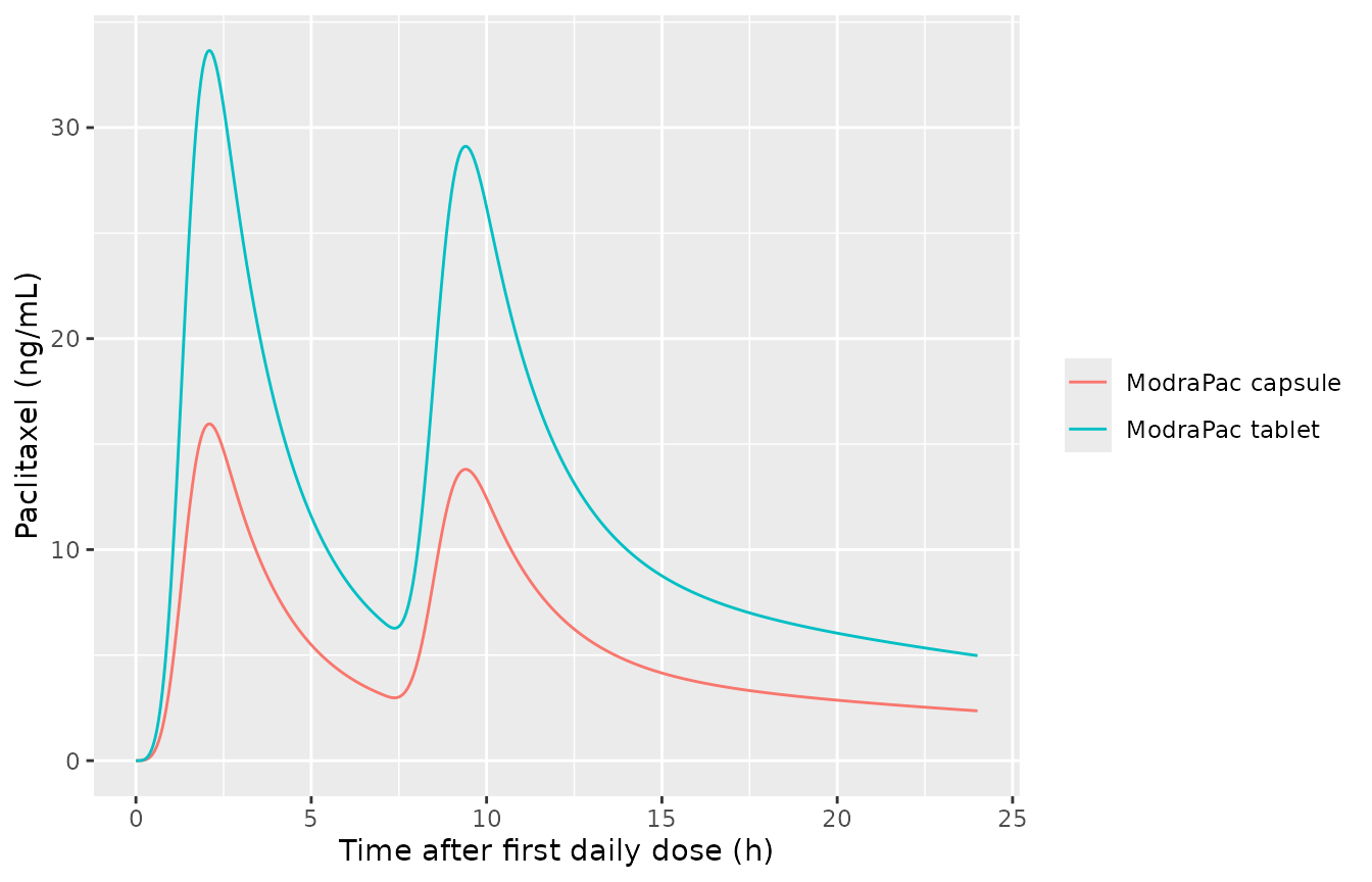
Day-1 profiles of the capsule and tablet at the RP2D (the paper’s Supplementary Figure S4, described in Results; the figure itself is not in the published supplementary file).
w3_tab |>
  dplyr::filter(time <= 72) |>
  dplyr::select(time, `Ritonavir (ng/mL)` = Cc_rtv, `CLint (L/h)` = clint) |>
  tidyr::pivot_longer(-time) |>
  ggplot(aes(time, value)) +
  geom_line() +
  facet_wrap(~name, scales = "free_y", ncol = 1) +
  labs(x = "Time (h)", y = NULL)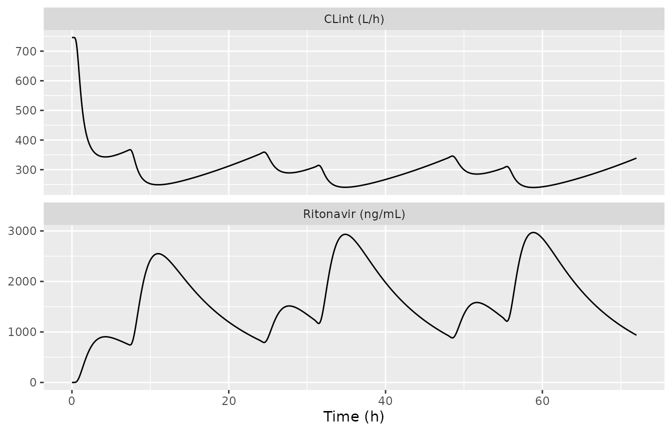
Ritonavir concentration and the resulting paclitaxel intrinsic clearance over the first 3 days of the RP2D regimen (compare Supplementary Figure S5, described in the Discussion).
TSP-1 response
w8 <- solve_typical(make_events(56, tab = 1L, cap = 0L, grid = 0.5))
ss8 <- w8[w8$time >= 24 * 55, ]
kin_rise <- range(ss8$Cc / (284 + ss8$Cc)) * 100
kin_rise
#> [1]  5.569961 22.228241
# Discussion: 5.4% to 22.0%.
stopifnot(abs(kin_rise[1] - 5.4) < 0.6, abs(kin_rise[2] - 22.0) < 1)
ggplot(w8, aes(time / 24, tsp1)) +
  geom_line() +
  geom_hline(yintercept = 43.8, linetype = "dotted") +
  labs(x = "Time (days)", y = "TSP-1 (ng/mL/10^6 platelets)")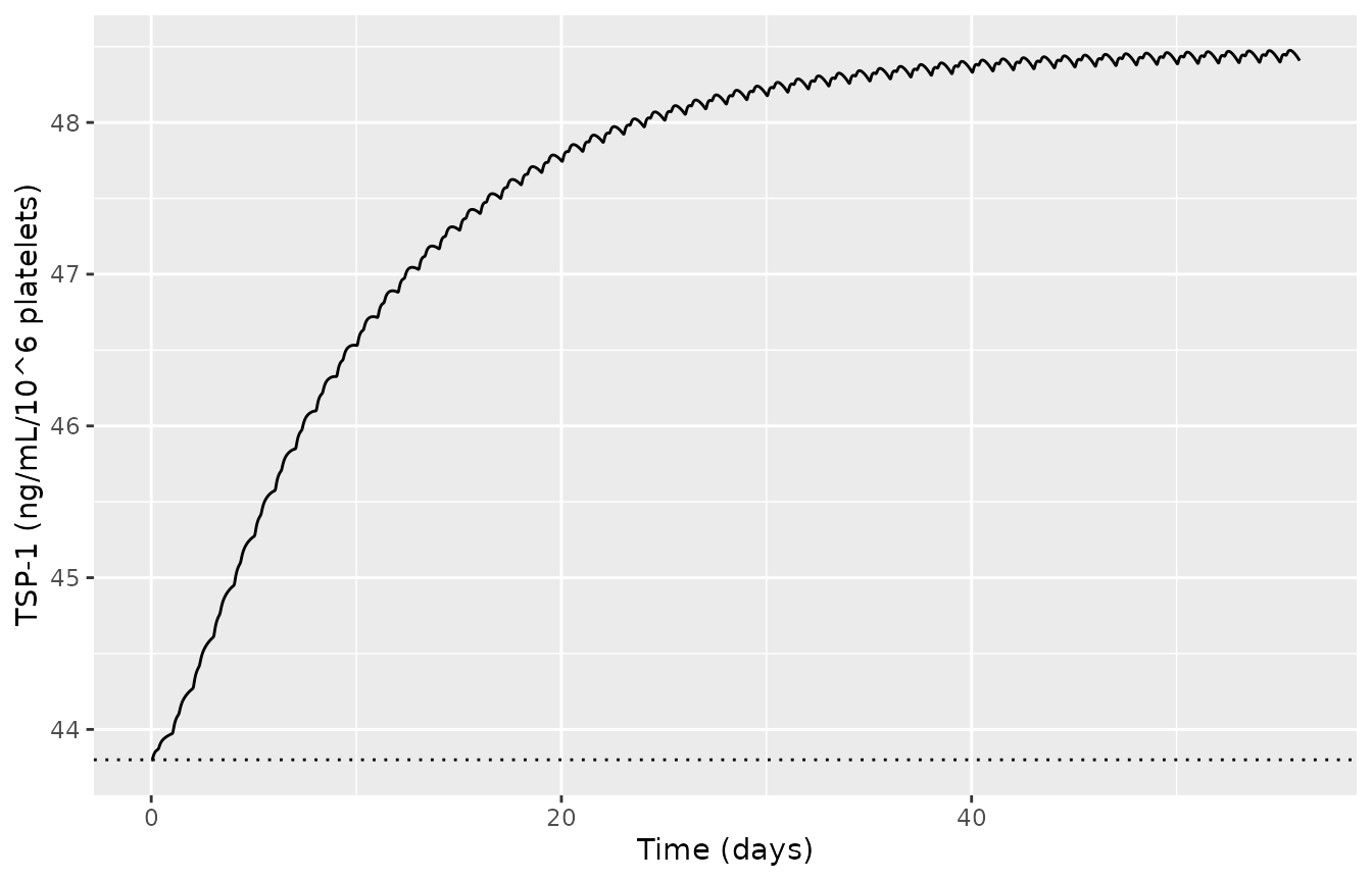
Typical TSP-1 time course during 8 weeks of the RP2D tablet regimen. The 233 h turnover time sets the approach to the new steady state.
Virtual cohort and PKNCA validation
Study 3 sampled PK over day 1 only. Two arms of 200 virtual patients
take the RP2D as capsule or tablet, with all between-subject,
between-occasion and residual variability. Each daily dose is its own
occasion (OCC 1 and 2), as in the paper. The paper reports
only typical-value AUC0-24, so the comparison below is between the
cohort median and the published typical value. With roughly 40-55% CV on
the absorption and bioavailability terms, these two need not coincide
exactly.
rxode2::rxSetSeed(20220707)
n_arm <- 200L
arms <- tibble::tibble(arm = c("ModraPac capsule", "ModraPac tablet"),
                       tab = c(0L, 1L), cap = c(1L, 0L), offset = c(0L, n_arm))
events <- dplyr::bind_rows(lapply(seq_len(nrow(arms)), function(a) {
  dplyr::bind_rows(lapply(seq_len(n_arm), function(i) {
    make_events(1, tab = arms$tab[a], cap = arms$cap[a], grid = 0.25,
                id = arms$offset[a] + i, occ = c(1L, 2L))
  })) |>
    dplyr::mutate(treatment = arms$arm[a])
}))
stopifnot(!anyDuplicated(unique(events[, c("id", "time", "evid", "cmt")])))
sim <- rxode2::rxSolve(mod, events, keep = "treatment", useLinCmt = FALSE,
                       returnType = "data.frame")
sim |>
  dplyr::group_by(time, treatment) |>
  dplyr::summarise(Q05 = quantile(Cc, 0.05), Q50 = median(Cc), Q95 = quantile(Cc, 0.95),
                   .groups = "drop") |>
  ggplot(aes(time, Q50)) +
  geom_ribbon(aes(ymin = Q05, ymax = Q95), alpha = 0.25) +
  geom_line() +
  facet_wrap(~treatment) +
  labs(x = "Time after first daily dose (h)", y = "Paclitaxel (ng/mL)")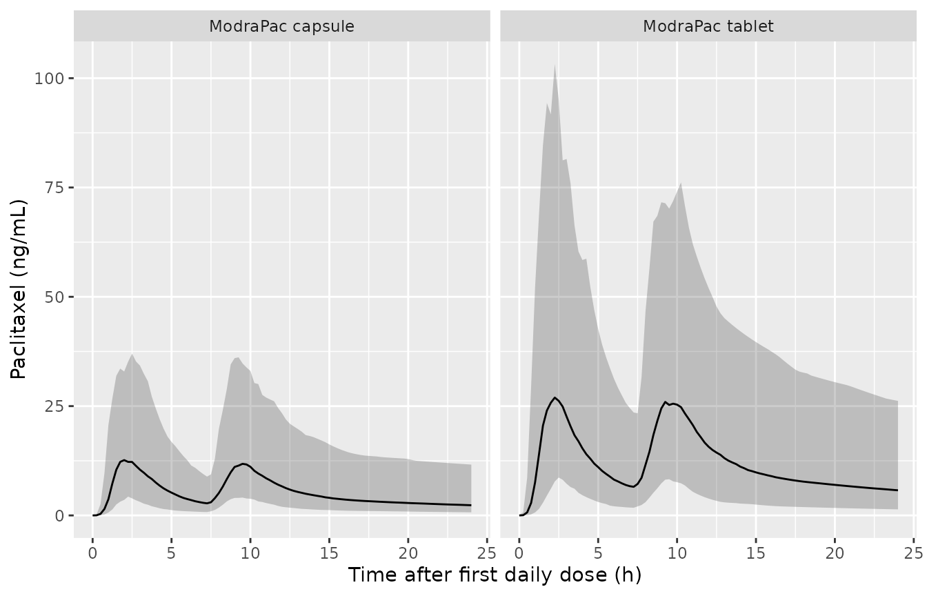
Day-1 paclitaxel concentrations (median and 5th-95th percentiles of individual predictions) for the capsule and tablet at the RP2D.
sim_nca <- sim |>
  dplyr::filter(!is.na(Cc)) |>
  dplyr::select(id, time, Cc, treatment)
sim_nca <- dplyr::bind_rows(
  sim_nca,
  sim_nca |> dplyr::distinct(id, treatment) |> dplyr::mutate(time = 0, Cc = 0)
) |>
  dplyr::distinct(id, treatment, time, .keep_all = TRUE) |>
  dplyr::arrange(id, treatment, time)
conc_obj <- PKNCA::PKNCAconc(sim_nca, Cc ~ time | treatment + id)
dose_df <- events |>
  dplyr::filter(evid == 1, cmt %in% c("depot1", "depot2")) |>
  dplyr::select(id, time, amt, treatment)
dose_obj <- PKNCA::PKNCAdose(dose_df, amt ~ time | treatment + id)
intervals <- data.frame(start = 0, end = 24, auclast = TRUE, cmax = TRUE, tmax = TRUE)
nca_res <- PKNCA::pk.nca(PKNCA::PKNCAdata(conc_obj, dose_obj, intervals = intervals))
published <- tibble::tribble(
  ~treatment, ~auclast,
  "ModraPac capsule", 131.4,
  "ModraPac tablet", 275.1
)
cmp <- nlmixr2lib::ncaComparisonTable(
  simulated = nca_res,
  reference = published,
  by = "treatment",
  units = c(auclast = "ng*h/mL", cmax = "ng/mL", tmax = "h"),
  tolerance_pct = 20
)
knitr::kable(cmp, caption = "Simulated cohort (median) vs published typical-value day-1 AUC0-24. * differs from reference by >20%.")| NCA parameter | treatment | Reference | Simulated | % diff |
|---|---|---|---|---|
| AUClast (ng*h/mL) | ModraPac capsule | 131 | 134 | +1.7% |
| AUClast (ng*h/mL) | ModraPac tablet | 275 | 314 | +14.3% |
auc_med <- as.data.frame(nca_res) |>
  dplyr::filter(PPTESTCD == "auclast") |>
  dplyr::group_by(treatment) |>
  dplyr::summarise(med = median(PPORRES), .groups = "drop") |>
  dplyr::left_join(published, by = "treatment")
auc_med
#> # A tibble: 2 × 3
#>   treatment          med auclast
#>   <chr>            <dbl>   <dbl>
#> 1 ModraPac capsule  134.    131.
#> 2 ModraPac tablet   314.    275.
# Realised: capsule +1.7%, tablet +14.3% versus the typical values. The cohort
# median differs from the typical-value prediction because exposure is a
# non-linear function of many log-normal terms (including the ritonavir
# variability), and each arm is one draw: with 200 subjects and an exposure
# CV of roughly 60%, the median carries a sampling SE of about 5%. The 30%
# bound leaves about 3 SE above the realised tablet value and still fails on
# a mis-transcribed rF, CLint0 or unit, which moves the median by > 50%.
stopifnot(nrow(auc_med) == 2, all(abs(auc_med$med / auc_med$auclast - 1) < 0.3))
# The tablet / capsule exposure ratio follows rF tablet / rF capsule = 2.1.
# The two arms are independent draws, so the ratio of medians has an SE of
# about 7%; the realised ratio is 2.35 (+12%), and the 25% bound is about
# 3.5 SE. Swapping the two rF values would move the ratio by > 75%.
ratio <- auc_med$med[auc_med$treatment == "ModraPac tablet"] /
  auc_med$med[auc_med$treatment == "ModraPac capsule"]
ratio
#> [1] 2.353196
stopifnot(abs(ratio / (0.97 / 0.46) - 1) < 0.25)
Assumptions and deviations
-
Eq. 9 is read literally. The printed
ka(t)is the Weibull density (it contains theexp(-(t/ALPHA)^BETA)factor), applied as a rate constant on the gut amount withtthe time after the last dose. The alternative, the Weibull hazard, would absorb the whole dose. The maintainers tested it against the paper’s own simulations. The hazard reading gives Tmax of 2.25 and 2.6 h (paper 2.1 and 2.4 h) and a day-1 tablet AUC0-24 of about 470 ug*h/L (paper 275.1). The literal reading reproduces both Tmax values exactly. -
Separate gut compartments for the two daily doses.
The paper estimates a separate ALPHA and rF for the first and second
daily dose, with time after the last dose as the Weibull clock. The
model doses them into
depot1anddepot2, so each dose’s 36.8% residue is absorbed when the next dose of the same daily slot restarts that compartment’s clock. The maintainers compared this with two alternatives:- One shared gut compartment (residue absorbed after the next dose of either slot) gives a day-1 AUC0-24 about 33% higher than published.
- Exact per-dose superposition (residue never absorbed) gives a steady-state Cmax of 52 ng/mL instead of 80.1.
- Ritonavir inverse Gaussian input. Yu 2020 Eq. 3 is a density input. It is encoded as its hazard on a gut amount, which is exact for a single dose (checked above) and conserves mass. When doses overlap, the residue of an earlier dose restarts on the new dose’s clock, as for paclitaxel. For the twice-daily RP2D, an exact superposition over all 42 ritonavir doses changed the steady-state paclitaxel Cmax and AUC0-504 by 0.2%.
- Residual day-1 AUC difference. Day-1 AUC0-24 is 5-6% above the published values for both formulations, while the steady-state quantities agree within 1-4%. Neither the ritonavir formulation nor the timing of ritonavir relative to paclitaxel in the paper’s simulation is stated. Both would only increase the AUC. The parameters were not adjusted.
-
Occasions. “Each dose administration was considered
an occasion”, and in the analysis data no subject had more than two PK
occasions. Two occasion slots are therefore encoded through
OCC(1 or 2; any other value switches the occasion etas off). This is used for the paclitaxel BOV on rF and for the Yu 2020 within-subject variability on the ritonavir MAT and absorption-time dispersion. rxode2 has no native occasion level, so these etas are multiplexed with indicators. rxode2 therefore warns that they are not mu-referenced. This only affects the speed of a future estimation run and does not change simulation. For multi-week stochastic simulations, draw a new occasion eta per dose (supply the eta columns on the dose rows). Otherwise doses beyond the second share the occasion-1 and occasion-2 draws. - Ritonavir variability. van Eijk 2022 fitted paclitaxel on each patient’s individual (Bayesian) ritonavir profile, or on typical ritonavir values when ritonavir was not sampled. For simulating new patients the model carries the Yu 2020 between-subject variability. Those values are held fixed because they are taken from Yu 2020 and not re-estimated.
-
Ritonavir formulation. Not reported for the van
Eijk studies. The Yu 2020 capsule reference is the default in this
article; the tablet (
FORM_RTV_TABLET = 1) raises ritonavir exposure by 6%. - CV% to variance. All CV% values were converted with omega^2 = log(1 + CV^2). The paper does not state the conversion.
- Supplementary material. The published supplementary file contains only a copy of Table 2. Supplementary Table 1 and Supplementary Figures S1-S5 are cited in the text but not available. No correction notice for this article was found as of 2026-10-03.
- Population. No demographic table is reported, so no covariate cohort could be built beyond formulation and dosing.