Acyclovir (Maximova 2022)
Source:vignettes/articles/Maximova_2022_acyclovir.Rmd
Maximova_2022_acyclovir.RmdModel and source
- Citation: Maximova N, Nistico D, Luci G, Simeone R, Piscianz E, Segat L, Barbi E, Di Paolo A. (2022). Population Pharmacokinetics of Intravenous Acyclovir in Oncologic Pediatric Patients. Front Pharmacol 13:865871. doi:10.3389/fphar.2022.865871
- Description: One-compartment population PK model for intravenous acyclovir in 120 oncologic children (age 0-18 years; mean weight 32.4 kg) receiving acyclovir prophylaxis or treatment for HSV/VZV infection during allogeneic HSCT or high-intensity chemotherapy, developed in NONMEM 7.4 from 374 therapeutic-drug-monitoring plasma concentrations (paired peak and trough samples on up to three occasions). Clearance scales allometrically with body weight (fixed exponent 0.75, reference 27.8 kg) and as a power function of Schwartz eGFR (reference 209.4 mL/min/1.73 m^2); volume scales linearly with body weight. Inter-individual variability on CL and V, inter-occasion variability on CL (three occasions), and proportional residual error.
- Article (open access): https://doi.org/10.3389/fphar.2022.865871
Population
Maximova 2022 enrolled 120 consecutive children (73 boys, 47 girls; age 8.6 +/- 5.0 years, median 9.5; weight 32.4 +/- 19.1 kg, median 27.8) treated for haematological malignancies at the IRCCS Burlo Garofolo in Trieste, Italy, between 2011 and 2020 (Table 1). Most were undergoing allogeneic haematopoietic stem cell transplantation. Ninety-four children received IV acyclovir as HSV/VZV prophylaxis and 26 as treatment of an active infection. Acyclovir was given every 6-8 h as a 60-min infusion (median starting daily dose 40.7 mg/kg/day, range 15.6-136.7). Doses were adjusted by therapeutic drug monitoring to keep Cmin above 0.5 mg/L and Cmax below 25 mg/L. Renal function was high for the age group: Schwartz eGFR 228.1 +/- 79.7 mL/min/1.73 m^2 (median 209.4).
The dataset holds 374 plasma concentrations. These are 187 peak/trough pairs, drawn 30 min after the end of infusion and 10 min before the next dose. They come from a first, second and third steady-state occasion in 120, 54 and 13 patients respectively.
The same information is available programmatically via
readModelDb("Maximova_2022_acyclovir")$population.
Source trace
| Equation / parameter | Value | Source location |
|---|---|---|
lcl (CL, 27.8 kg, eGFR 209.4) |
6.184 L/h | Table 2, Final model, CL row (bootstrap median 6.186) |
lvc (V, 27.8 kg) |
18.942 L | Table 2, Final model, V row (bootstrap median 19.129) |
e_crcl_cl |
1.627 | Table 2, ‘EGFR on CL’ row |
e_wt_cl (held constant) |
0.75 | Table 2 footnote equation (WGT/27.8)^0.75
|
e_wt_vc (held constant) |
1 | Table 2 footnote equation (WGT/27.8)^1
|
etalcl variance |
log(1 + 0.452^2) = 0.186 | Table 2, IIV CL = 45.2% |
etalvc variance |
log(1 + 0.567^2) = 0.279 | Table 2, IIV V = 56.7% |
etaiov_cl_1..3 variance |
log(1 + 0.20^2) = 0.0392 | Table 2, IOV CL = 20.0% |
propSd |
sqrt(0.181) = 0.425 | Table 2, ‘Residual variability’ = 0.181 (proportional; Results, POP/PK Modeling) |
| One-compartment model, first-order elimination, IV infusion | – | Methods, Pharmacokinetic Modeling; Results, POP/PK Modeling |
CL = 6.184 * (eGFR/209.4)^1.627 * (WT/27.8)^0.75 * exp(eta1 + IOV) |
– | Table 2 footnote (printed with + signs; see
Assumptions) |
V = 18.942 * (WT/27.8) * exp(eta2) |
– | Table 2 footnote |
| Reference values 209.4 mL/min/1.73 m^2 and 27.8 kg | – | Table 1 medians |
Typical-value check against a closed form
A one-compartment model at steady state under a repeated 1-h infusion has a closed-form concentration profile. Writing it from the Table 2 numbers, rather than from the model file, catches transcription errors in the clearance, volume, covariate exponent and units.
mod <- rxode2::rxode2(readModelDb("Maximova_2022_acyclovir"))
#> ℹ parameter labels from comments will be replaced by 'label()'
#> Warning: some etas defaulted to non-mu referenced, possible parsing error: etaiov_cl_1, etaiov_cl_2, etaiov_cl_3
#> as a work-around try putting the mu-referenced expression on a simple line
mod_typ <- rxode2::zeroRe(mod)
#> Warning: some etas defaulted to non-mu referenced, possible parsing error: etaiov_cl_1, etaiov_cl_2, etaiov_cl_3
#> as a work-around try putting the mu-referenced expression on a simple line

# Child at eGFR = 250 mL/min/1.73 m^2, WT = 40 kg: both covariates away from
# their references so that every exponent is exercised.
wt <- 40
egfr <- 250
cl_cf <- 6.184 * (egfr / 209.4)^1.627 * (wt / 27.8)^0.75
v_cf <- 18.942 * (wt / 27.8)
k_cf <- cl_cf / v_cf
dose <- 20 * wt
tau <- 6
tinf <- 1
rate <- dose / tinf
ss_conc <- function(t) {
  # t = time since the start of the last infusion (0 <= t <= tau)
  cend <- rate / cl_cf * (1 - exp(-k_cf * tinf)) / (1 - exp(-k_cf * tau))
  ifelse(
    t <= tinf,
    rate / cl_cf * (1 - exp(-k_cf * t)) +
      cend * exp(-k_cf * (tau - tinf)) * exp(-k_cf * t),
    cend * exp(-k_cf * (t - tinf))
  )
}

ndose <- 25
t_last <- (ndose - 1) * tau
obs_t <- t_last + c(0.5, 1, 1.5, 3, 5.83, 6)
ev_cf <- data.frame(
  id = 1L,
  time = c((seq_len(ndose) - 1) * tau, obs_t),
  evid = c(rep(1L, ndose), rep(0L, length(obs_t))),
  amt = c(rep(dose, ndose), rep(0, length(obs_t))),
  rate = c(rep(rate, ndose), rep(0, length(obs_t))),
  cmt = "central",
  WT = wt,
  CRCL = egfr,
  OCC = 1L
) |>
  arrange(time, desc(evid))

sim_cf <- rxode2::rxSolve(mod_typ, ev_cf, returnType = "data.frame") |>
  mutate(closed_form = ss_conc(time - t_last), pct_diff = 100 * (Cc / closed_form - 1))
#> ℹ omega/sigma items treated as zero: 'etalcl', 'etalvc', 'etaiov_cl_1', 'etaiov_cl_2', 'etaiov_cl_3'

sim_cf |>
  transmute(
    "Time since infusion start (h)" = time - t_last,
    "rxode2 Cc (mg/L)" = signif(Cc, 4),
    "Closed form (mg/L)" = signif(closed_form, 4),
    "Difference (%)" = signif(pct_diff, 2)
  ) |>
knitr::kable(caption = "Typical-value steady state, 20 mg/kg q6h 1-h infusion, WT 40 kg, eGFR 250.")| Time since infusion start (h) | rxode2 Cc (mg/L) | Closed form (mg/L) | Difference (%) |
|---|---|---|---|
| 0.50 | 16.300 | 16.300 | 6.2e-05 |
| 1.00 | 26.670 | 26.670 | 1.1e-04 |
| 1.50 | 21.860 | 21.860 | 3.1e-04 |
| 3.00 | 12.040 | 12.040 | 1.1e-04 |
| 5.83 | 3.907 | 3.907 | 4.7e-04 |
| 6.00 | 3.651 | 3.651 | 4.5e-04 |
Virtual cohort
The cohort reproduces the Table 1 demographics. Body weight and eGFR are drawn from log-normal distributions with the Table 1 mean and SD; this places the weight median at 27.9 kg and the eGFR median at 215 mL/min/1.73 m^2, close to the observed 27.8 kg and 209.4. Each child receives 10 mg/kg every 6 h as a 1-h infusion, about the cohort’s median starting dose of 40.7 mg/kg/day. All observations are on occasion 1.
rxode2::rxSetSeed(20220414)
set.seed(20220414)
n_sub <- 200

lnorm_par <- function(m, s) {
  sdlog <- sqrt(log(1 + (s / m)^2))
  c(meanlog = log(m) - sdlog^2 / 2, sdlog = sdlog)
}
p_wt <- lnorm_par(32.4, 19.1)
p_gfr <- lnorm_par(228.1, 79.7)

cohort <- tibble(
  id = seq_len(n_sub),
  WT = pmin(pmax(rlnorm(n_sub, p_wt[["meanlog"]], p_wt[["sdlog"]]), 6), 100),
  CRCL = pmin(pmax(rlnorm(n_sub, p_gfr[["meanlog"]], p_gfr[["sdlog"]]), 60), 500),
  OCC = 1L,
  treatment = "10 mg/kg q6h"
)

tau <- 6
ndose <- 16
t_last <- (ndose - 1) * tau
obs_grid <- t_last + sort(unique(c(seq(0, 6, by = 0.25), 1.5, 5.83)))

doses <- cohort |>
  tidyr::crossing(dose_i = seq_len(ndose)) |>
  mutate(
    time = (dose_i - 1) * tau, evid = 1L, amt = 10 * WT, rate = amt / 1,
    cmt = "central"
  ) |>
  select(-dose_i)
obs <- cohort |>
  tidyr::crossing(time = obs_grid) |>
  mutate(evid = 0L, amt = 0, rate = 0, cmt = "central")
events <- bind_rows(doses, obs) |>
  arrange(id, time, desc(evid))

sim <- rxode2::rxSolve(mod, events, keep = c("treatment", "WT", "CRCL"), returnType = "data.frame")
Steady-state peak and trough against the TDM data
Figure 2 and the Results text summarise the measured concentrations. At occasion 1, Cmax 30 min after the end of infusion was 7.6 +/- 5.4 mg/L. Cmin 10 min before the next dose was 1.0 +/- 1.1 mg/L on the 6-h schedule.
pt <- sim |>
  filter(abs(time - (t_last + 1.5)) < 1e-6 | abs(time - (t_last + 5.83)) < 1e-6) |>
  mutate(sample = ifelse(time - t_last < 3, "Peak (1.5 h)", "Trough (5.83 h)")) |>
  group_by(sample) |>
  summarise(
    "Simulated mean +/- SD (mg/L)" = sprintf("%.2f +/- %.2f", mean(sim), sd(sim)),
    "Simulated median (mg/L)" = sprintf("%.2f", median(sim)),
    sim_median = median(sim),
    .groups = "drop"
  ) |>
  mutate("Observed mean +/- SD (mg/L)" = c("7.6 +/- 5.4", "1.0 +/- 1.1"))
pt |>
  select(-sim_median) |>
  rename("Sample" = sample) |>
knitr::kable(caption = "Simulated (with residual error) vs observed occasion-1 peak and trough, 10 mg/kg q6h.")| Sample | Simulated mean +/- SD (mg/L) | Simulated median (mg/L) | Observed mean +/- SD (mg/L) |
|---|---|---|---|
| Peak (1.5 h) | 14.01 +/- 11.93 | 10.69 | 7.6 +/- 5.4 |
| Trough (5.83 h) | 4.68 +/- 7.55 | 1.96 | 1.0 +/- 1.1 |
The model, with the Table 2 estimates, predicts peaks and troughs above the measured values: the peak by roughly twofold and the trough by several-fold. The paper reports the same bias. Figure 3A shows a regression of observations on population predictions that lies well below the line of identity, and the Results note “an overprediction during the first few hours after the dose”. This is a property of the published fit, not of the transcription. The typical-value check above confirms that the model file reproduces the Table 2 numbers.
sim |>
  mutate(tad = time - t_last) |>
  group_by(tad) |>
  summarise(
    med = median(Cc), lo = quantile(Cc, 0.05), hi = quantile(Cc, 0.95),
    .groups = "drop"
  ) |>
  ggplot(aes(tad, med)) +
  geom_ribbon(aes(ymin = lo, ymax = hi), alpha = 0.25) +
  geom_line() +
  geom_vline(xintercept = c(1.5, 5.83), linetype = "dashed") +
  scale_y_log10() +
  labs(x = "Time after start of infusion (h)", y = "Acyclovir Cc (mg/L)")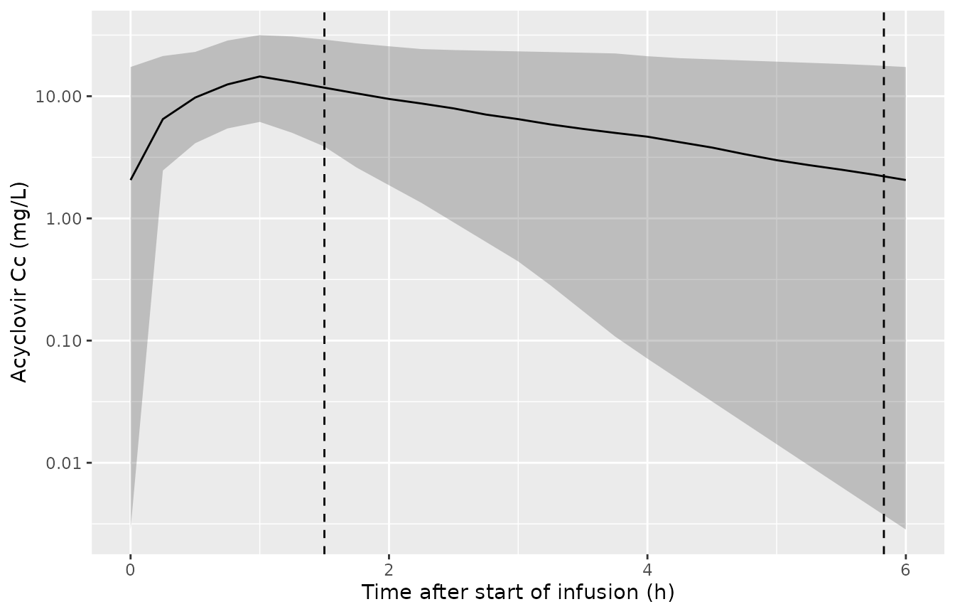
Simulated steady-state profiles, 10 mg/kg q6h 1-h infusion (median and 5th-95th percentiles), with the TDM sampling times of Figure 2 marked.
PKNCA validation
sim_nca <- sim |>
  filter(!is.na(Cc)) |>
  select(id, time, Cc, treatment)

conc_obj <- PKNCA::PKNCAconc(sim_nca, Cc ~ time | treatment + id)
dose_df <- events |>
  filter(evid == 1) |>
  select(id, time, amt, treatment)
dose_obj <- PKNCA::PKNCAdose(dose_df, amt ~ time | treatment + id, route = "intravascular", duration = 1)

intervals <- data.frame(
  start = t_last, end = t_last + tau,
  cmax = TRUE, tmax = TRUE, cmin = TRUE, auclast = TRUE, half.life = TRUE
)
nca_res <- PKNCA::pk.nca(PKNCA::PKNCAdata(conc_obj, dose_obj, intervals = intervals))

published <- tibble::tribble(
  ~treatment, ~auclast, ~half.life,
  "10 mg/kg q6h", 23.3, 1.237
)
cmp <- nlmixr2lib::ncaComparisonTable(
  simulated = nca_res,
  reference = published,
  by = "treatment",
  params = c("cmax", "cmin", "auclast", "half.life"),
  units = c(cmax = "mg/L", cmin = "mg/L", auclast = "h*mg/L", half.life = "h"),
  tolerance_pct = 20
)
knitr::kable(cmp, caption = "Simulated steady-state NCA (median) vs Table 3 empirical-Bayes medians. * differs from reference by >20%.")| NCA parameter | treatment | Reference | Simulated | % diff |
|---|---|---|---|---|
| AUClast (h*mg/L) | 10 mg/kg q6h | 23.3 | 41.7 | +79.0%* |
| t½ (h) | 10 mg/kg q6h | 1.24 | 1.8 | +45.3%* |
Both rows differ from Table 3 by more than 20%. Table 3 summarises the individual empirical Bayes estimates: CL 14.0 +/- 5.5 L/h (median 14.6), V 25.4 +/- 8.7 L (median 26.1), kel 0.574 1/h and t1/2 1.364 h. Those estimates sit far above the Table 2 typical values. CL is about 2.3-fold the typical 6.184 L/h, which is much more than the eGFR and weight distribution of the cohort or the log-normal mean shift can explain. The typical-value half-life of the Table 2 model is about 2.1 h, against a Table 3 median of 1.24 h, and the AUC follows the clearance. The model file keeps the Table 2 estimates. They agree with the bootstrap medians, so they are the reported final estimates. The Table 3 offset is recorded below as a known deviation.
indiv <- sim |>
  distinct(id, cl, vc) |>
  mutate(kel = cl / vc, thalf = log(2) / kel)
tibble(
  "Parameter" = c("CL (L/h)", "V (L)", "kel (1/h)", "t1/2 (h)"),
  "Simulated median" = signif(c(median(indiv$cl), median(indiv$vc), median(indiv$kel), median(indiv$thalf)), 3),
  "Table 3 median (EBE)" = c(14.6, 26.1, 0.558, 1.237)
) |>
knitr::kable(caption = "Simulated individual parameters vs Table 3 empirical-Bayes medians.")| Parameter | Simulated median | Table 3 median (EBE) |
|---|---|---|
| CL (L/h) | 6.750 | 14.600 |
| V (L) | 16.700 | 26.100 |
| kel (1/h) | 0.386 | 0.558 |
| t1/2 (h) | 1.800 | 1.237 |
Dosing-regimen simulations (Tables 6 and 7)
The paper simulated 1,000 children per regimen, with body weight fixed at 27.8 kg and eGFR drawn from a normal distribution with mean 228.1 and SD 79.7 mL/min/1.73 m^2. Results were stratified at 250 mL/min/1.73 m^2. The simulation below follows that design with 200 children per regimen. Cmin is read just before the next dose and Cmax at the end of the infusion.
rxode2::rxSetSeed(865871)
set.seed(865871)
n_arm <- 200
regimens <- tribble(
  ~regimen, ~mgkg, ~tau, ~tinf,
  "10 mg/kg q6h 1 h", 10, 6, 1,
  "20 mg/kg q6h 1 h", 20, 6, 1,
  "30 mg/kg q6h 1 h", 30, 6, 1,
  "10 mg/kg q8h 1 h", 10, 8, 1,
  "20 mg/kg q8h 1 h", 20, 8, 1,
  "30 mg/kg q8h 1 h", 30, 8, 1,
  "20 mg/kg q6h 2 h", 20, 6, 2,
  "20 mg/kg q6h 3 h", 20, 6, 3,
  "10 mg/kg q8h continuous", 10, 8, 8
) |>
  mutate(arm = row_number())

subj <- regimens |>
  tidyr::crossing(k = seq_len(n_arm)) |>
  mutate(id = (arm - 1L) * n_arm + k, WT = 27.8, OCC = 1L)
subj$CRCL <- pmax(rnorm(nrow(subj), 228.1, 79.7), 30)

t_end <- 72
pta_dose <- subj |>
  group_by(id) |>
  reframe(
    time = seq(0, t_end, by = tau[1]), amt = mgkg[1] * WT[1],
    rate = mgkg[1] * WT[1] / tinf[1]
  ) |>
  mutate(evid = 1L)
pta_obs <- subj |>
  mutate(t0 = floor(t_end / tau) * tau) |>
  select(id, t0, tau, tinf) |>
  tidyr::crossing(which = c("cmax", "cmin")) |>
  mutate(time = ifelse(which == "cmax", t0 + tinf, t0 + tau), evid = 0L, amt = 0, rate = 0) |>
  select(id, time, evid, amt, rate)
pta_events <- bind_rows(pta_dose, pta_obs) |>
  left_join(select(subj, id, WT, CRCL, OCC, regimen), by = "id") |>
  mutate(cmt = "central") |>
  arrange(id, time, desc(evid))

pta_sim <- rxode2::rxSolve(mod, pta_events, keep = c("regimen", "CRCL"), returnType = "data.frame") |>
  group_by(id, regimen, CRCL) |>
  summarise(cmax = max(ipredSim), cmin = ipredSim[which.max(time)], .groups = "drop") |>
  mutate(egfr_group = ifelse(CRCL <= 250, "eGFR <= 250", "eGFR > 250"))

pta <- pta_sim |>
  group_by(regimen, egfr_group) |>
  summarise(
    n = n(),
    cmin_056 = 100 * mean(cmin > 0.56),
    cmin_1125 = 100 * mean(cmin > 1.125),
    cmax_25 = 100 * mean(cmax > 25),
    .groups = "drop"
  )

paper <- tribble(
  ~regimen, ~egfr_group, ~p_056, ~p_1125, ~p_25,
  "10 mg/kg q6h 1 h", "eGFR <= 250", 50.9, 35.2, 1.0,
  "20 mg/kg q6h 1 h", "eGFR <= 250", 62.5, 50.9, 28.6,
  "30 mg/kg q6h 1 h", "eGFR <= 250", 67.9, 57.8, 67.3,
  "10 mg/kg q6h 1 h", "eGFR > 250", 37.8, 22.2, 0.6,
  "20 mg/kg q6h 1 h", "eGFR > 250", 50.6, 37.9, 21.3,
  "30 mg/kg q6h 1 h", "eGFR > 250", 59.0, 44.8, 55.6,
  "10 mg/kg q8h 1 h", "eGFR <= 250", 31.2, 19.1, 1.0,
  "20 mg/kg q8h 1 h", "eGFR <= 250", 44.4, 31.2, 25.0,
  "30 mg/kg q8h 1 h", "eGFR <= 250", 50.1, 39.6, 63.8,
  "10 mg/kg q8h 1 h", "eGFR > 250", 20.1, 11.1, 0.6,
  "20 mg/kg q8h 1 h", "eGFR > 250", 32.8, 20.1, 20.6,
  "30 mg/kg q8h 1 h", "eGFR > 250", 37.6, 26.8, 52.4,
  "20 mg/kg q6h 2 h", "eGFR <= 250", 69.3, 57.4, 2.5,
  "20 mg/kg q6h 3 h", "eGFR <= 250", 76.9, 66.0, 0.6,
  "20 mg/kg q6h 2 h", "eGFR > 250", 59.2, 44.3, 0.6,
  "20 mg/kg q6h 3 h", "eGFR > 250", 65.6, 54.8, 0.0
)

pta |>
  left_join(paper, by = c("regimen", "egfr_group")) |>
  mutate(regimen = factor(regimen, levels = regimens$regimen)) |>
  arrange(regimen, egfr_group) |>
  transmute(
    "Regimen" = regimen,
    "eGFR group" = egfr_group,
    "n" = n,
    "Cmin > 0.56, sim (%)" = round(cmin_056, 1),
    "Cmin > 0.56, paper (%)" = p_056,
    "Cmin > 1.125, sim (%)" = round(cmin_1125, 1),
    "Cmin > 1.125, paper (%)" = p_1125,
    "Cmax > 25, sim (%)" = round(cmax_25, 1),
    "Cmax > 25, paper (%)" = p_25
  ) |>
knitr::kable(caption = "Probability of target attainment: model simulation vs Maximova 2022 Tables 6 and 7.")| Regimen | eGFR group | n | Cmin > 0.56, sim (%) | Cmin > 0.56, paper (%) | Cmin > 1.125, sim (%) | Cmin > 1.125, paper (%) | Cmax > 25, sim (%) | Cmax > 25, paper (%) |
|---|---|---|---|---|---|---|---|---|
| 10 mg/kg q6h 1 h | eGFR <= 250 | 123 | 91.1 | 50.9 | 82.9 | 35.2 | 30.9 | 1.0 |
| 10 mg/kg q6h 1 h | eGFR > 250 | 77 | 53.2 | 37.8 | 31.2 | 22.2 | 0.0 | 0.6 |
| 20 mg/kg q6h 1 h | eGFR <= 250 | 127 | 94.5 | 62.5 | 90.6 | 50.9 | 78.0 | 28.6 |
| 20 mg/kg q6h 1 h | eGFR > 250 | 73 | 63.0 | 50.6 | 52.1 | 37.9 | 32.9 | 21.3 |
| 30 mg/kg q6h 1 h | eGFR <= 250 | 114 | 94.7 | 67.9 | 91.2 | 57.8 | 95.6 | 67.3 |
| 30 mg/kg q6h 1 h | eGFR > 250 | 86 | 67.4 | 59.0 | 53.5 | 44.8 | 86.0 | 55.6 |
| 10 mg/kg q8h 1 h | eGFR <= 250 | 117 | 81.2 | 31.2 | 75.2 | 19.1 | 20.5 | 1.0 |
| 10 mg/kg q8h 1 h | eGFR > 250 | 83 | 34.9 | 20.1 | 24.1 | 11.1 | 2.4 | 0.6 |
| 20 mg/kg q8h 1 h | eGFR <= 250 | 119 | 82.4 | 44.4 | 75.6 | 31.2 | 75.6 | 25.0 |
| 20 mg/kg q8h 1 h | eGFR > 250 | 81 | 51.9 | 32.8 | 37.0 | 20.1 | 29.6 | 20.6 |
| 30 mg/kg q8h 1 h | eGFR <= 250 | 123 | 86.2 | 50.1 | 78.9 | 39.6 | 95.9 | 63.8 |
| 30 mg/kg q8h 1 h | eGFR > 250 | 77 | 45.5 | 37.6 | 35.1 | 26.8 | 76.6 | 52.4 |
| 20 mg/kg q6h 2 h | eGFR <= 250 | 119 | 95.0 | 69.3 | 91.6 | 57.4 | 64.7 | 2.5 |
| 20 mg/kg q6h 2 h | eGFR > 250 | 81 | 76.5 | 59.2 | 69.1 | 44.3 | 14.8 | 0.6 |
| 20 mg/kg q6h 3 h | eGFR <= 250 | 119 | 96.6 | 76.9 | 93.3 | 66.0 | 46.2 | 0.6 |
| 20 mg/kg q6h 3 h | eGFR > 250 | 81 | 71.6 | 65.6 | 63.0 | 54.8 | 7.4 | 0.0 |
| 10 mg/kg q8h continuous | eGFR <= 250 | 124 | 100.0 | NA | 100.0 | NA | 10.5 | NA |
| 10 mg/kg q8h continuous | eGFR > 250 | 76 | 100.0 | NA | 97.4 | NA | 0.0 | NA |
The levels in Tables 6 and 7 cannot be reproduced from the Table 2 estimates. With Table 2 the eGFR <= 250 group exceeds the trough targets far more often than the paper reports, for example roughly 90% against 50.9% for Cmin > 0.56 mg/L at 10 mg/kg q6h. The gap between the two eGFR groups is also much wider than in the paper. Neither alternative reading of the footnote equation closes the gap, and the paper’s own trough levels correspond to a clearance near the Table 3 empirical-Bayes values. The paper’s continuous-infusion result shows the same offset. It reports a steady-state Cmin of 3.18 +/- 1.69 mg/L at eGFR <= 250 for 10 mg/kg every 8 h. The same regimen in the simulation above gives a median of 7.3 mg/L in that group.
The direction of every regimen effect in Tables 6 and 7 is reproduced, and those directions are checked below. They depend on the structure of the model, not on the level of clearance. Four checks use the simulated cohort: lower attainment in the eGFR > 250 group, lower trough attainment at q8h than at q6h (pooled over the three doses and both eGFR groups), more Cmax > 25 mg/L at higher doses, and fewer toxic peaks as the infusion is prolonged. Each difference must exceed three binomial standard errors. Trough attainment is close to 100% in the eGFR <= 250 group, so the rise in trough with longer infusions is checked on the typical child instead (WT 27.8 kg, eGFR 209.4), where it is deterministic.
pick <- function(reg, grp, col) {
  pta[[col]][pta$regimen == reg & pta$egfr_group == grp]
}
n_of <- function(reg, grp) pta$n[pta$regimen == reg & pta$egfr_group == grp]
# Three binomial SEs of the difference of two proportions (in %), using the
# pooled proportion -- a margin that admits draw-to-draw noise.
se3 <- function(p1, p2, n1, n2) {
  p <- (p1 + p2) / 200
  3 * 100 * sqrt(max(p * (1 - p), 0.01) * (1 / n1 + 1 / n2))
}
trend <- function(reg1, grp1, reg2, grp2, col) {
  p1 <- pick(reg1, grp1, col)
  p2 <- pick(reg2, grp2, col)
  (p1 - p2) > se3(p1, p2, n_of(reg1, grp1), n_of(reg2, grp2))
}
lo <- "eGFR <= 250"
hi <- "eGFR > 250"

# q6h vs q8h, pooled over 10/20/30 mg/kg 1-h infusions and both eGFR groups.
pooled <- pta_sim |>
  filter(grepl("1 h$", regimen)) |>
  mutate(interval = sub(".* (q[68]h) .*", "\\1", regimen)) |>
  group_by(interval) |>
  summarise(n = n(), cmin_056 = 100 * mean(cmin > 0.56), .groups = "drop")
p6 <- pooled$cmin_056[pooled$interval == "q6h"]
p8 <- pooled$cmin_056[pooled$interval == "q8h"]

# Typical child: trough and peak by infusion length, 20 mg/kg q6h.
typ_inf <- lapply(c(1, 2, 3), function(ti) {
  ev <- data.frame(
    id = 1L,
    time = c(seq(0, 72, by = 6), 72 + ti, 78),
    evid = c(rep(1L, 13), 0L, 0L),
    amt = c(rep(20 * 27.8, 13), 0, 0),
    rate = c(rep(20 * 27.8 / ti, 13), 0, 0),
    cmt = "central", WT = 27.8, CRCL = 209.4, OCC = 1L
  )
  out <- rxode2::rxSolve(mod_typ, ev, returnType = "data.frame")
  data.frame(tinf = ti, cmax = out$Cc[1], cmin = out$Cc[2])
}) |>
  bind_rows()
#> ℹ omega/sigma items treated as zero: 'etalcl', 'etalvc', 'etaiov_cl_1', 'etaiov_cl_2', 'etaiov_cl_3'
#> ℹ omega/sigma items treated as zero: 'etalcl', 'etalvc', 'etaiov_cl_1', 'etaiov_cl_2', 'etaiov_cl_3'
#> ℹ omega/sigma items treated as zero: 'etalcl', 'etalvc', 'etaiov_cl_1', 'etaiov_cl_2', 'etaiov_cl_3'
knitr::kable(signif(typ_inf, 3), caption = "Typical child (27.8 kg, eGFR 209.4), 20 mg/kg q6h: Cmax at the end of infusion and Cmin at 6 h, by infusion length (h).")| tinf | cmax | cmin |
|---|---|---|
| 1 | 29.2 | 5.70 |
| 2 | 25.1 | 6.80 |
| 3 | 21.8 | 8.18 |
checks <- c(
  egfr_group = trend("20 mg/kg q6h 1 h", lo, "20 mg/kg q6h 1 h", hi, "cmin_056"),
  q6h_vs_q8h = (p6 - p8) > se3(p6, p8, pooled$n[1], pooled$n[2]),
  dose_cmax = trend("30 mg/kg q6h 1 h", lo, "10 mg/kg q6h 1 h", lo, "cmax_25"),
  infusion_cmax = trend("20 mg/kg q6h 1 h", lo, "20 mg/kg q6h 3 h", lo, "cmax_25"),
  # Deterministic typical-value solve: a strict ordering is safe here.
  infusion_cmin = all(diff(typ_inf$cmin) > 0) && all(diff(typ_inf$cmax) < 0)
)
checks
#>    egfr_group    q6h_vs_q8h     dose_cmax infusion_cmax infusion_cmin
#>          TRUE          TRUE          TRUE          TRUE          TRUE
stopifnot(all(checks))
Assumptions and deviations
-
Footnote equation typesetting. The Table 2 footnote
prints
CL = [6.184 + (eGFR/209.4)^1.627 + (WGT/27.8)^0.75]^(eta1 + IOV)andV = [18.942 + (WGT/27.8)^1]^eta2. The maintainers read the+signs as multiplication and the eta superscripts as exponentials. This gives the standard power-covariate, log-normal-eta form that the Results describe: eGFR “on CL” and “allometric scaling” of body weight. Read literally, weight would change V by about 1 L over the whole cohort range, and raising a typical value to the power of eta would give CL = 1 L/h at eta = 0. Neither reading is plausible. The additive reading also fails to reproduce Tables 3, 6 and 7. - Typical values vs the paper’s derived outputs. The Table 2 estimates sit well below the paper’s empirical-Bayes summaries (Tables 3-5: CL 14.0 L/h, V 25.4 L) and below the clearance implied by its simulations (Tables 6-7). They are also below the clearance implied by its measured troughs (Figure 2). The paper itself shows population predictions above the observations (Figure 3A, CWRES vs time in Figure 3D). The model file keeps the Table 2 values, which the bootstrap medians (6.186 L/h, 19.129 L) confirm are the reported estimates. Users should expect typical-value simulations to overpredict acyclovir peaks in this population roughly twofold and troughs several-fold. The paper does not give enough detail to find the source of the inconsistency, and no correction notice had been published as of 2026-10-01.
-
IIV and IOV scale. Table 2 gives IIV and IOV as
percentages. They were converted to log-scale variances as
log(1 + CV^2). The Results quote an IIV of 46.4% and the Discussion 46.3%, each within 1.2 points of the table’s 45.2%. Neither theomega^2 = CV^2nor thelog(1 + CV^2)reading reproduces those prose figures exactly. - Residual error scale. Table 2 gives ‘Residual variability’ as the bare number 0.181 under a proportional error model. The IIV rows are printed as percentages, so this row was read as the NONMEM SIGMA variance, giving a proportional SD of 0.425. The pcVPC (Figure 4) supports this reading: at 1.5 h the simulated 5th percentile is a small fraction of the median (roughly 0.1-0.25). The maintainers simulated a reference child (27.8 kg, eGFR 209.4, 10 mg/kg q6h) with the Table 2 IIV and IOV. With a 0.425 SD the 5th percentile falls near 0.26 times the median, and with a 0.181 SD near 0.5 times.
-
Inter-occasion variability. IOV on CL is encoded
with an
OCCcolumn (1-3) and three occasion etas sharing one variance, after the paper’s three TDM occasions. SettingOCCoutside 1-3 turns IOV off. - Virtual cohort. Body weight and eGFR come from log-normal distributions with the Table 1 mean and SD, truncated to 6-100 kg and 60-500 mL/min/1.73 m^2. The individual records were not published. The regimen simulations follow the paper’s own design: WT 27.8 kg and eGFR from a normal distribution with mean 228.1 and SD 79.7, floored at 30.
- Cmax and Cmin definitions in the regimen simulations. Cmax is read at the end of the infusion and Cmin at the end of the dosing interval. The paper does not say at which times its simulated Cmax and Cmin were read.