Model and source
- Citation: Jain L, Woo S, Gardner ER, Dahut WL, Kohn EC, Kummar S, Mould DR, Giaccone G, Yarchoan R, Venitz J, Figg WD. Population pharmacokinetic analysis of sorafenib in patients with solid tumours. Br J Clin Pharmacol. 2011;72(2):294-305. doi:10.1111/j.1365-2125.2011.03963.x.
- Description: One-compartment population PK model for orally administered sorafenib in patients with solid tumours (Jain 2011). Absorption is described by an Erlang-style chain of four catenary GI transit compartments downstream of an upstream absorption depot, all linked by a single first-order rate constant ka (mean absorption transit time MAT = 5 / ka). Enterohepatic recirculation is modelled by routing a fraction Fent of the drug leaving the central compartment into a gallbladder reservoir, with periodic release back to the most distal transit compartment gated by a smooth Hill switch Ehc = tad^40 / (tad^40 + t’^40), where tad is the time since the most recent dose; release becomes essentially full once tad exceeds the gallbladder-emptying onset time t’. The irreversible elimination rate constant ke equals the biliary excretion rate constant kb (= CL/V) per the published assumption kb = ke. Body weight is the only retained covariate (allometric exponent fixed to 1 on V/F, reference weight 80 kg).
- Article: Br J Clin Pharmacol 2011;72(2):294-305. https://doi.org/10.1111/j.1365-2125.2011.03963.x
Population
The model was developed in 111 adults with metastatic solid tumours enrolled across five NCI phase I / II trials: metastatic castrate-resistant prostate cancer (PC, n = 46), non-small-cell lung cancer (NSCLC, n = 18), colorectal cancer (CRC, n = 18), other solid tumours (ST, n = 28), and Kaposi’s sarcoma (KS, n = 2). The cohort spanned 30.3-84.9 years of age (median 63.9), 50.1-132.5 kg of body weight (median 81.4 kg), 81% Caucasian, 11% African-American, and was 69% male (Table 2, p. 297). All patients received either 200 mg or 400 mg sorafenib twice daily in continuous cycles as monotherapy or in combination with cetuximab, bevacizumab, or a protease inhibitor. Genotyping for CYP3A4*1B, CYP3A5*3C, UGT1A9*3, and UGT1A9*5 single-nucleotide polymorphisms was performed for all patients (UGT1A9*5 was non-polymorphic in the cohort). Plasma was sampled at 0, 0.25, 0.5, 1, 2, 4, 6, 8, and 12 h post first dose with one additional sample 12 h after the second dose, and at steady-state in selected patients; 1249 sorafenib concentrations were used for PPK model building, of which 3.3% were below the LLOQ and reported as actual values (Methods and Results, p. 297-298). One patient was excluded from analysis because of extremely low plasma concentrations (approximately 30-fold lower than other patients).
The same information is available programmatically via
readModelDb("Jain_2011_sorafenib")$population.
Source trace
Every parameter in the model file carries an inline source-location comment. The table below collects the entries in one place.
| Equation / parameter | Value | Source location |
|---|---|---|
lmtt (mean absorption transit time MAT) |
1.98 h | Table 3, MAT row (CI 1.75-2.25 h); ka = 5 / MAT per Table 3 footnote |
lcl (apparent clearance CL/F) |
8.13 L/h | Table 3, CL/F row (CI 6.98-10.7 L/h) |
lvc (apparent central volume V/F at WT = 80 kg) |
213 L | Table 3, V/F row (CI 196-232 L) |
lkehc (EHC release rate constant) |
0.857 1/h | Table 3, kEhc row (CI 0.478-1.26) |
ltprime (gallbladder-emptying onset time t’) |
6.13 h | Table 3, t’ row (CI 5.78-7.34); paper footnote: “absolute time post dose administration at which EHC starts” |
fent (fraction of dose undergoing EHC) |
0.498 | Table 3, Fent row (CI 0.464-0.498); derived from estimated Ferts via Fent = 1 / (1 + Ferts) per Table 3 footnote |
e_wt_vc (allometric exponent on V/F, FIXED) |
1.0 | Results p. 300: “modelled as a power function with the exponent fixed to 1” |
| IIV CL/F (omega^2 = log(1 + 0.180^2) = 0.0319) | 18.0% CV | Table 3, IIV CL/F row |
| IIV V/F (omega^2 = log(1 + 0.687^2) = 0.3866) | 68.7% CV | Table 3, IIV V/F row |
| IIV ka (omega^2 = log(1 + 0.619^2) = 0.3240) | 61.9% CV | Table 3, IIV ka row (same variance applies on the log MAT scale) |
| Correlation CL/F <-> V/F (cov = 0.0864) | 0.778 | Table 3, “Correlation CL/F-V/F” row |
| Proportional residual error | 51.4% CV | Table 3, “Proportional residual error” row (CI 45.6-56%) |
| Additive residual error | 1.0003e-3 mg/L | Table 3, “Additive residual error” row |
| Transit absorption: dA0/dt = -ka A0; dAi/dt = ka (A(i-1) - Ai) for i = 1..3 | – | Equations (4)-(6), p. 299 |
| dA4/dt = ka (A3 - A4) + Ehc kEhc Agb | – | Equation (7), p. 299 |
| dAcc/dt = ka A4 - Fent kb Acc - (1-Fent) (CL/V) Acc | – | Equation (8), p. 299; kb = ke per Results p. 300 |
| dAgb/dt = Fent kb Acc - Ehc kEhc Agb | – | Equation (9), p. 299 |
| Ehc gating: Ehc = (t - DT)^40 / ((t - DT)^40 + t’^40) | – | Equation (10), p. 300; Figure 2 visualises the resulting square-wave switch |
| Combined residual error: ln(Cij) = ln(Cij_hat) + sqrt(eps_p^2 + eps_a^2 / Cij_hat^2) | – | Equation (1), p. 297 |
Virtual cohort
Original observed data are not publicly available. The virtual cohort below mirrors the two clinical doses Jain 2011 studied: 200 mg BID and 400 mg BID. Body weights are drawn from a log-normal distribution with median 81 kg and an inter-individual CV that approximates the Table 2 total-cohort range (50-132 kg).
set.seed(20110301)

n_per_dose <- 50L
weight_log_sd <- 0.20  # roughly matches the Table 2 weight spread

make_cohort <- function(n, dose_mg, label, id_offset = 0L) {
  tibble(
    id     = id_offset + seq_len(n),
    WT     = round(81 * exp(rnorm(n, 0, weight_log_sd)), 1),
    dose   = dose_mg,
    cohort = label
  )
}

demo <- bind_rows(
  make_cohort(n_per_dose, dose_mg = 200, label = "200 mg BID",
              id_offset = 0L),
  make_cohort(n_per_dose, dose_mg = 400, label = "400 mg BID",
              id_offset = n_per_dose)
)
stopifnot(!anyDuplicated(demo$id))
Simulation
Each subject receives sorafenib twice daily (q12h) for 14 days. Sampling follows the Methods description (Pharmacokinetic sampling and sample analysis, p. 296): a dense grid of 0, 0.25, 0.5, 1, 2, 4, 6, 8, 12 h relative to the first dose, plus a 12-h-post-second-dose sample, plus selected steady-state samples in a final-day window.
init_grid <- c(0, 0.25, 0.5, 1, 2, 4, 6, 8, 12, 24)
ss_grid   <- 312 + c(0, 0.25, 0.5, 1, 2, 4, 6, 8, 12)
# Combine dense initial + final-day windows; PKNCA recipe drives the
# steady-state interval [312, 324] off the last dose.

build_events <- function(demo, obs_grid) {
  doses <- demo |>
    tidyr::crossing(dose_index = 0:27) |>           # 28 doses = 14 days BID
    mutate(time = dose_index * 12,
           amt  = dose,
           evid = 1L,
           cmt  = "depot") |>
    select(id, time, amt, evid, cmt, cohort, WT)
  obs <- demo |>
    tidyr::crossing(time = obs_grid) |>
    mutate(amt = NA_real_, evid = 0L, cmt = NA_character_) |>
    select(id, time, amt, evid, cmt, cohort, WT)
  bind_rows(doses, obs) |> arrange(id, time, desc(evid))
}

events_dense <- build_events(demo,
                             obs_grid = c(init_grid, ss_grid))
events_typ   <- build_events(demo,
                             obs_grid = seq(0, 336, by = 0.25))
mod <- rxode2::rxode2(readModelDb("Jain_2011_sorafenib"))
#> ℹ parameter labels from comments will be replaced by 'label()'

sim_pop <- rxode2::rxSolve(mod, events = events_dense,
                           keep = c("cohort", "WT"),
                           nStud = 1) |>
  as.data.frame()

mod_typical <- mod |> rxode2::zeroRe()
sim_typ <- rxode2::rxSolve(mod_typical, events = events_typ,
                           keep = c("cohort", "WT")) |>
  as.data.frame()
#> ℹ omega/sigma items treated as zero: 'etalcl', 'etalvc', 'etalmtt'
#> Warning: multi-subject simulation without without 'omega'
Replicate published figures
Figure 1A – typical plasma concentration vs. time after the first dose
Figure 1A of Jain 2011 shows individual sorafenib concentration-time profiles from four representative patients over the first 24 h, with the characteristic delayed absorption and a second peak around 6-8 h attributable to enterohepatic recirculation. The typical-value profile below mirrors that shape.
fig1A <- sim_typ |>
  filter(time > 0, time <= 24) |>
  group_by(cohort, time) |>
  summarise(Cc = mean(Cc), .groups = "drop")

ggplot(fig1A, aes(time, Cc, colour = cohort)) +
  geom_line(linewidth = 0.8) +
  scale_x_continuous(breaks = seq(0, 24, by = 4)) +
  scale_y_continuous(limits = c(0, NA)) +
  labs(x = "Time post first dose (h)",
       y = "Sorafenib concentration (mg/L)",
       colour = "Dose group",
       title = "Typical-value plasma profile after the first oral dose",
       caption = "Replicates Figure 1A of Jain 2011 (single representative profile per dose group).")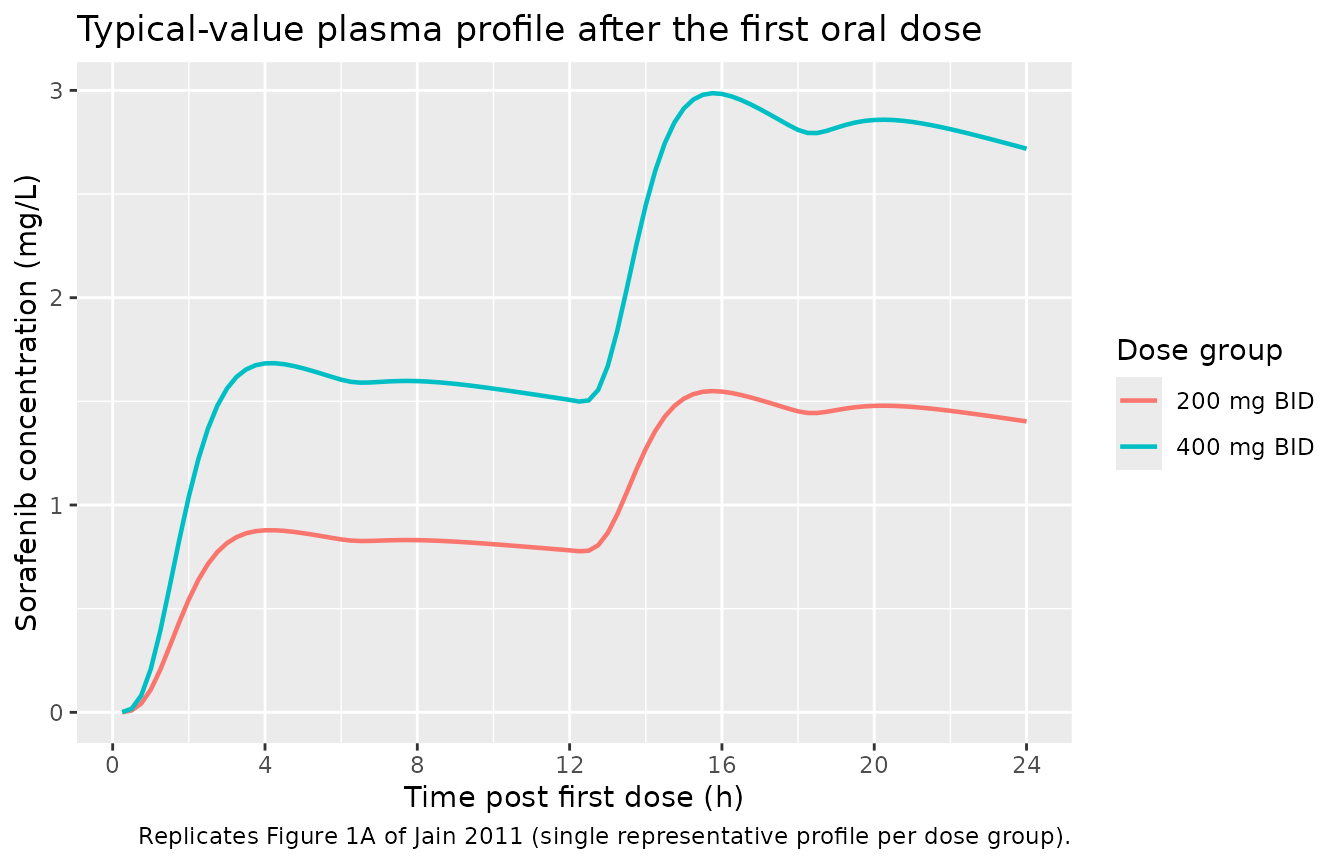
Replicates Figure 1A of Jain 2011: typical-value sorafenib plasma concentration vs. time after the first oral dose. The delayed absorption (peak ~3-5 h) plus the second peak around 8-10 h reflect the four GI transit compartments and the gallbladder-emptying enterohepatic recycling encoded by Ehc(t).
Figure 2 – the Ehc switch function
Figure 2 of Jain 2011 plots Ehc(t) over multiple dosing intervals to show that the smooth Hill switch behaves as a square wave: 0 immediately after each dose, rising to ~1 once tad exceeds t’ (= 6.13 h), then resetting at the next dose. The chunk below extracts the same trace from the typical simulation.
fig2 <- sim_typ |>
  filter(time <= 48, cohort == "400 mg BID") |>
  select(time, Ehc) |>
  distinct()

ggplot(fig2, aes(time, Ehc)) +
  geom_line(linewidth = 0.7) +
  scale_x_continuous(breaks = seq(0, 48, by = 6)) +
  scale_y_continuous(limits = c(-0.05, 1.1)) +
  labs(x = "Time (h)",
       y = "Ehc switch (unitless)",
       title = "Enterohepatic recycling on/off function",
       caption = "Replicates Figure 2 of Jain 2011 (t' = 6.13 h, Hill exponent = 40).")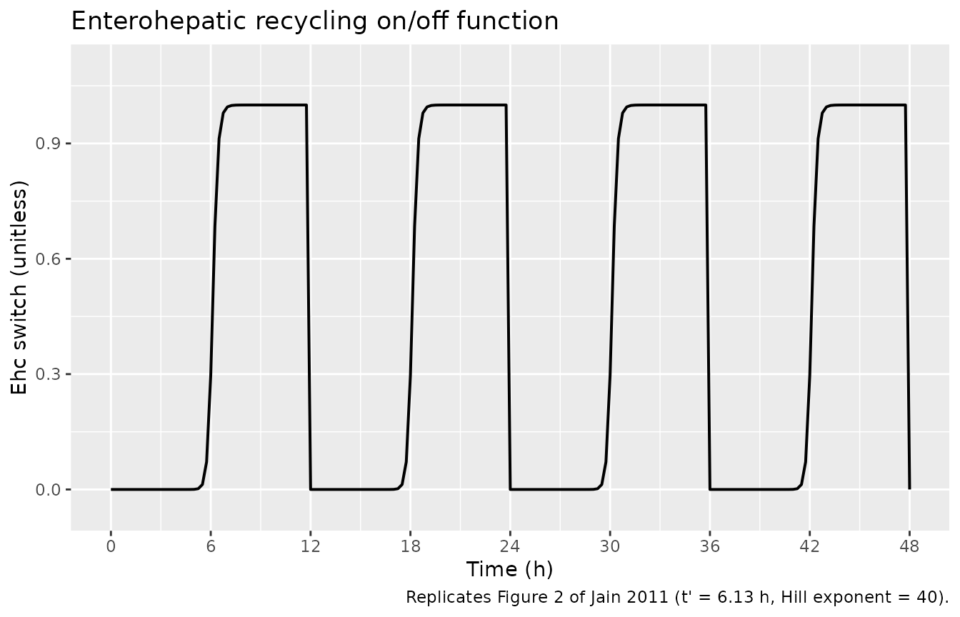
Replicates Figure 2 of Jain 2011: the Hill-shaped Ehc switch over the first 48 h of BID dosing. Ehc rises sharply from ~0 to ~1 once tad exceeds the gallbladder-emptying onset time t’ = 6.13 h, then resets at each subsequent dose.
Figure 4 – steady-state stochastic VPC, dose-normalised
Figure 4 of Jain 2011 shows the visual predictive check after the first dose (panel A) and at steady state (panel B), with concentrations dose-normalised so the 200 mg and 400 mg BID curves overlay. The chunk below reproduces the steady-state panel.
ss_window <- tibble(
  ss_start = 312,
  ss_end   = 324
)

vpc_ss <- sim_pop |>
  filter(time >= ss_window$ss_start, time <= ss_window$ss_end) |>
  mutate(dose             = if_else(cohort == "200 mg BID", 200, 400),
         time_in_interval = time - ss_window$ss_start,
         Cc_dose_norm     = Cc / dose) |>
  group_by(time_in_interval) |>
  summarise(Q05 = quantile(Cc_dose_norm, 0.05, na.rm = TRUE),
            Q50 = quantile(Cc_dose_norm, 0.50, na.rm = TRUE),
            Q95 = quantile(Cc_dose_norm, 0.95, na.rm = TRUE),
            .groups = "drop")

ggplot(vpc_ss, aes(time_in_interval, Q50)) +
  geom_ribbon(aes(ymin = Q05, ymax = Q95), alpha = 0.3) +
  geom_line(linewidth = 0.8) +
  scale_x_continuous(breaks = seq(0, 12, by = 2)) +
  scale_y_continuous(limits = c(0, NA)) +
  labs(x = "Time in steady-state dosing interval (h)",
       y = "Dose-normalised concentration (mg/L per mg dose)",
       title = "Steady-state dose-normalised VPC",
       caption = "Replicates Figure 4B of Jain 2011 (last BID dosing interval, days 13-14).")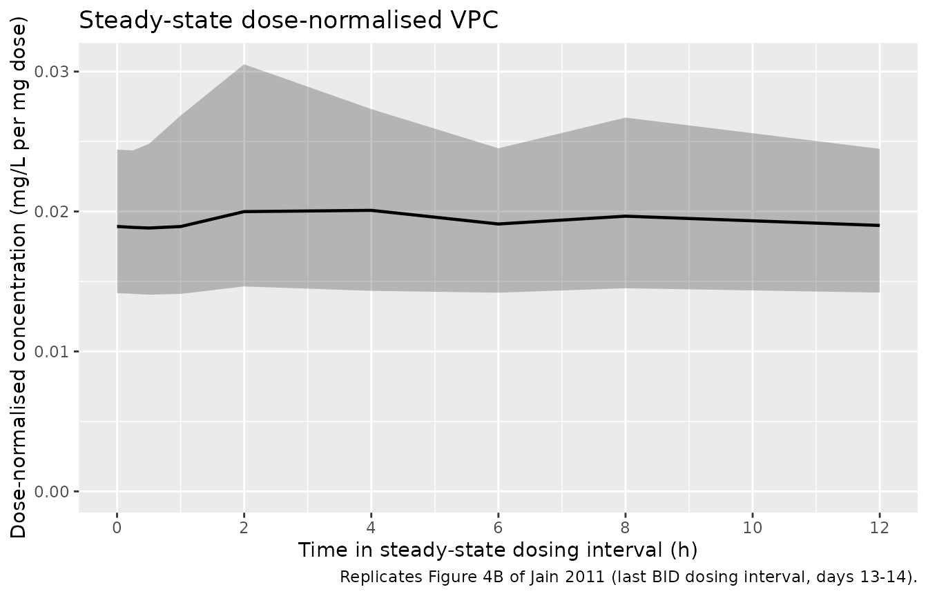
Replicates Figure 4B of Jain 2011: steady-state stochastic VPC, dose-normalised. Median and 5th/95th percentile envelope of dose-normalised sorafenib concentration over the final BID dosing interval.
PKNCA validation
Jain 2011 does not tabulate NCA-derived Cmax, Tmax, AUC, or half-life values per dose group – the publication is a population-PK paper whose primary outputs are the structural parameters in Table 3. The PKNCA block below computes the steady-state Cmax,ss, Tmax,ss, AUC0-tau (tau = 12 h), and average concentration over the final BID dosing interval for each dose group as model documentation. Qualitative agreement is checked against the prose-reported sorafenib exposure range cited in the introduction (AUC %CV 5-83%, Cmax %CV 33-88% across the published 200 / 400 mg BID dose levels; p. 295).
nca_input <- sim_pop |>
  filter(!is.na(Cc), time >= 312, time <= 324) |>
  select(id, time, Cc, cohort)

# Anchor a time = 312 (start of interval) sample per (id, cohort); the
# rxSolve grid already includes 312, but the defensive bind_rows is the
# documented PKNCA recipe pattern.
nca_input <- bind_rows(
  nca_input,
  nca_input |> distinct(id, cohort) |>
    mutate(time = 312, Cc = 0)
) |>
  distinct(id, cohort, time, .keep_all = TRUE) |>
  arrange(id, cohort, time)

dose_df <- events_dense |>
  filter(evid == 1L, time == 312) |>
  select(id, time, amt, cohort)

conc_obj <- PKNCA::PKNCAconc(nca_input, Cc ~ time | cohort + id,
                             concu = "mg/L", timeu = "hour")
dose_obj <- PKNCA::PKNCAdose(dose_df, amt ~ time | cohort + id,
                             doseu = "mg")

intervals <- data.frame(
  start   = 312,
  end     = 324,
  cmax    = TRUE,
  tmax    = TRUE,
  cmin    = TRUE,
  auclast = TRUE,
  cav     = TRUE,
  ctrough = TRUE
)

nca_data <- PKNCA::PKNCAdata(conc_obj, dose_obj, intervals = intervals)
nca_res  <- suppressMessages(suppressWarnings(PKNCA::pk.nca(nca_data)))

knitr::kable(
  summary(nca_res),
  caption = "Steady-state NCA over the final BID dosing interval (50 subjects per dose group). Cmax,ss, Tmax,ss, and AUC0-12 reflect the EHC second peak; expect Tmax,ss to land in the 4-8 h window rather than the absorption peak around 3-5 h."
)| Interval Start | Interval End | cohort | N | AUClast (hour*mg/L) | Cmax (mg/L) | Cmin (mg/L) | Tmax (hour) | Cav (mg/L) | Ctrough (mg/L) |
|---|---|---|---|---|---|---|---|---|---|
| 312 | 324 | 200 mg BID | 50 | 46.1 [19.7] | 4.09 [23.1] | 3.64 [18.0] | 3.00 [1.00, 12.0] | 3.84 [19.7] | NC |
| 312 | 324 | 400 mg BID | 50 | 94.0 [20.4] | 8.32 [25.0] | 7.45 [18.3] | 4.00 [2.00, 12.0] | 7.84 [20.4] | NC |
The dose-proportional ratio of Cmax and AUC0-12 between 400 mg BID and 200 mg BID should be very close to 2.0 in this model (no saturable-absorption / saturable-clearance terms were fit). Departures from 2.0 in the table above point to noise from the 50-subject cohort size rather than a structural mismatch.
Assumptions and deviations
-
Parameter values are paper-derived. Every entry in
ini()carries its Table 3 page-3 source-location comment. No parameter value was carried in from an upstream task, an author email, or a digitised figure. -
Body weight is the only retained covariate. Sex,
BSA, age, serum albumin, ALT, creatinine clearance, and the four
genotype indicators (CYP3A4*1B, CYP3A5*3C, UGT1A9*3, UGT1A9*5) were
screened during forward addition but did not survive backward
elimination (Results, p. 300). They are documented in
covariatesDataExcludedso the provenance is preserved without triggering “declared but unused” convention warnings. -
Allometric exponent on V/F is FIXED to 1. Per
Results p. 300 (“…modelled as a power function with the exponent fixed
to 1”). The paper notes that this only explained ~4% of IIV in V/F (the
other 65% of V/F IIV remains unaccounted for). Encoded as
e_wt_vc <- fixed(1.0). -
kb = ke assumption. The paper attempted to estimate
kb (biliary excretion rate constant) and ke (irreversible elimination
rate constant) separately and found the joint model unstable; the
assumption kb = ke (both equal to CL/V) was retained for stability
(Results, p. 300). The packaged model implements this via a single
kel = cl/vcterm, with the gallbladder receiving thefentfraction of the central-compartment outflow and the rest eliminated irreversibly. -
MAT vs. ka parameterisation. The paper estimates
mean absorption transit time MAT (Table 3) and reports the IIV on the
linear-scale ka. Because MAT = 5 / ka (Table 3 footnote), the variance
on log(MAT) equals the variance on log(ka), so the canonical
lmttparameterisation with IIVetalmtt ~ log(1 + 0.619^2)is mathematically identical to alkaparameterisation with the same variance. Insidemodel(),ka <- 5 / mttrecovers the absorption rate constant used by the four-transit-compartment chain. -
Inter-occasion variability (IOV) on CL/F not
modelled. Table 3 reports IOV CL/F = 47.7% CV with
stratification by initial dose vs. steady state. Because IOV requires
per-occasion event-time stratification that nlmixr2 / rxode2 does not
natively support inside the
ini()/model()body without externalOCCcovariate columns, the packaged model carries IIV CL/F only (18.0% CV) and documents IOV here. The reported IOV magnitude (47.7%) is larger than the residual IIV (18%) and may dominate within-subject variability; users intending to simulate intra-individual variability should add an OCC-stratified perturbation onetalclexternally. -
EHC gating uses
tad(). Equation (10) isEhc = (t - DT)^40 / ((t - DT)^40 + t'^40)where DT is the time of the most recent dose. rxode2 exposes the time since the most recent dose via thetad()helper, so the model usestad_h <- tad()andEhc <- tad_h^40 / (tad_h^40 + tprime^40). The Hill exponent of 40 makes Ehc effectively a step function (rising from < 1e-3 at tad = 5 h to ~0.98 at tad = 6.75 h with t’ = 6.13 h), reproducing the square-wave Figure 2 pattern without the numerical-differentiation problems that would arise with an explicit step. - kb = kEhc was not stable, and is not assumed. The paper also attempted to set kb = kEhc but the joint model was numerically unstable. The packaged model uses the published parameterisation: kb = kel and kEhc is a separate freely-estimated parameter (Table 3 row kEhc = 0.857 1/h).
-
Logit-transformed Fent stored as the back-transformed point
estimate. Jain 2011 estimated the logit of Fent to keep it
bounded in (0, 1) during FOCEI; Table 3 reports the back-transformed
median 0.498 with a 95% CI of (0.464, 0.498) – visibly skewed because
the estimated logit was very close to zero. The packaged model stores
fent = 0.498directly as a bounded unitless parameter; the logit transformation was a numerical convenience during estimation, not a structural feature of the model. - Vignette uses 50 subjects per dose group. Small enough to render the vignette in well under the 5-minute pkgdown gate, large enough to give stable VPC percentiles and PKNCA summaries. Jain 2011 used a 10 000-virtual-patient simulation for the published VPC (Results, p. 298).
- NCA reference values not tabulated in the source. Jain 2011 does not report cohort-specific Cmax / Tmax / AUC point estimates; only the prose-described %CV ranges (AUC 5-83%, Cmax 33-88%) and the published prior-study ranges cited in the abstract. The PKNCA block therefore shows simulated values for documentation rather than a side-by-side comparison table against published numbers.