Deferasirox iron chelation (Sakares 2025)
Source:vignettes/articles/Sakares_2025_deferasirox.Rmd
Sakares_2025_deferasirox.RmdModel and source
- Citation: Sakares W, Udomnilobol U, Pan X, Yampayon K, Ekwattanakit S, Viprakasit V, Limwongse C, Srichairatanakool S, Teerawonganan P, Kunsa-ngiem S, Khaowroongrueng V, Techatanawat I, Prueksaritanont T, Yodsurang V. Bridging Pharmacokinetics and Pharmacodynamics: A PBPK/PD Model-Based Approach for Deferasirox Dosing in Transfusion-Dependent Thalassemia. Clin Transl Sci. 2025;18(9):e70355. doi:10.1111/cts.70355 (PMID 40965322; PMCID PMC12445128).
- Description: PBPK/PD (iron-chelation PD layer only). Two-compartment iron-homeostasis model (chelatable iron in the blood volume, storage iron in the liver) with deferasirox (DFX) binding chelatable iron at 2:1 stoichiometry and the DFX-iron complex eliminated first-order, in adults with transfusion-dependent thalassaemia (TDT) and healthy adults (Sakares 2025). Uptake from chelatable to storage iron is Michaelis-Menten plus a linear chelatable-iron-driven term; efflux from storage iron is Michaelis-Menten scaled by a hepcidin-like factor that rises with liver iron concentration (LIC) and falls with chelatable iron. TDT lowers dietary iron absorption and adds a transfusional iron input. The paper’s DFX PK layer is a Simcyp V22 whole-body PBPK model (ADAM absorption, retrograde enzyme kinetics, platform physiology) whose organ volumes, blood flows and partition coefficients are not printed, so it is not reproduced: total plasma DFX is supplied as the time-varying covariate CP_DEFERASIROX_UM. The output liver_iron is liver iron concentration (mg Fe/g dry weight). No inter-individual variability or residual error is reported; the model is deterministic.
- Article: https://doi.org/10.1111/cts.70355 (open access, PMC12445128)
Sakares 2025 couples a Simcyp V22 whole-body PBPK model of deferasirox (DFX) to a two-compartment iron-homeostasis model written as a custom Lua module in the simulator. The PBPK layer uses the ADAM absorption model, enzyme kinetics back-calculated by Simcyp’s retrograde tool, and the simulator’s “Sim-Healthy Volunteer” physiology adapted for thalassaemia. The paper prints none of the organ volumes, blood flows or tissue partition coefficients, so that layer cannot be rebuilt outside the simulator.
The iron model is fully specified (Eq. 1-6 and Table 1), and that is
what Sakares_2025_deferasirox contains. Total plasma DFX
enters as the time-varying covariate CP_DEFERASIROX_UM
(umol/L). The model has three states:
-
cfe, the chelatable iron pool (non-transferrin-bound and labile iron), with the total blood volume of 5.40 L; -
sfe, the storage iron pool (ferritin and haemosiderin), with the liver volume of 1.69 L; -
complex, the DFX-iron complex.
The output liver_iron is liver iron concentration in mg
Fe/g dry weight: liver_iron = sfe / 2886.2.
Population
The PD layer was calibrated (COPASI 4.44) to iron turnover and LIC progression in healthy adults and patients with transfusion-dependent thalassaemia (TDT). It was then verified against LIC after 6 or 12 months of DFX in four Caucasian TDT datasets (Piga 2006, Cappellini 2006) and two Thai TDT datasets from the Siriraj Thalassemia Center (Supplementary Table S1). Across the TDT datasets, baseline LIC was 2.5-31.44 mg/g and transfusional iron loading 0.31-0.62 mg/kg/day; ages were 18-66 years. Healthy subjects were assigned the reference LIC of 0.98 mg/g and no transfusional iron (Table S1 footnote).
Source trace
| Element | Value | Source |
|---|---|---|
d/dt(cfe) |
absorption + transfusion - loss - uptake + efflux * Vol_sFe/Vol_cFe - net complex formation | Eq. 3 (Eq. 1 without DFX) |
d/dt(sfe) |
uptake * Vol_cFe/Vol_sFe - efflux | Eq. 4 (= Eq. 2) |
d/dt(complex) |
kon * cFe * (DFX * fu)^2 - (koff + keli) * complex | Eq. 6 |
| uptake | Vmax,uptake * cFe/(Km,uptake + cFe) + ka * cFe | Eq. 1-4 |
| efflux | Vmax,efflux * sFe/(Km,efflux + sFe) * (a * sFe/2886.2 * exp(-b * cFe))^c | Eq. 1-4 |
kin_fe / kin_fe_tdt
|
0.28 / 0.07 umol/L/h | Table 1, k_in (Healthy / TDT) |
kout_fe |
0.28 umol/L/h | Table 1, k_out |
vol_sfe, vol_cfe
|
1.69 L, 5.40 L | Table 1 |
vmax_uptake, km_uptake,
k_cfe_uptake
|
0.306687 umol/L/h, 15.2 umol/L, 1e-6 1/h | Table 1 |
vmax_efflux, km_efflux
|
43 umol/L/h, 1e6 umol/L | Table 1 |
hep_a, hep_b, hep_c
|
1.66 g/mg, 0.036 L/umol, 0.135 | Table 1 |
sfe_per_lic |
2886.2 umol/L per mg/g | Eq. 1-4 (= 2828.48 / 0.98, Table 1 and Table S1) |
kon, koff, keli
|
200, 0.96, 0.4 | Table 1 |
fu |
0.004 | Table 1 |
sfe(0) |
LIVER_IRON_BL * 2886.2 | Table 1 initial storage iron; Table S1 baseline LIC |
cfe(0) = cfe0
|
2.2853 umol/L | Derived: healthy steady state of Eq. 1-2 (see Assumptions) |
kblood |
TRANSF_IRON_MGKGD * WT / 55.845 * 1000 / 24 / Vol_cFe | Table 1 k_blood “Various”; Table S1 / S6 loadings; unit conversion (see Assumptions) |
WT used below |
Table S2 weight-height-age equations | Table S2 |
Simulation helpers
The model needs a DFX concentration profile. To exercise it, this vignette adds a simple one-compartment oral DFX driver ahead of the iron model by model piping. The driver is per kilogram, so a dose in mg/kg gives umol/L directly. Its apparent clearance comes from the paper’s own simulated AUC for 20 mg/kg in TDT patients (Table S4, dataset 9: 570.05 umol/Lh). Its absorption rate and apparent volume are solved so that the profile also matches the simulated Cmax of 53.40 umol/L at a Tmax of about 3 h (read from Figure 4a). The driver is a validation input only. It is not part of the packaged model, and it holds DFX at the concentration the paper’s PBPK model would give after* chelation, which is what the covariate represents.
mw_dfx <- 373.4 # g/mol, Table 1
dose_ref <- 20 / mw_dfx * 1000 # umol/kg for 20 mg/kg
cl_f <- dose_ref / 570.05 # L/h/kg, Table S4 dataset 9 simulated AUC

driver_obj <- function(p) {
  ka <- exp(p[1])
  v <- exp(p[2])
  ke <- cl_f / v
  tmax <- log(ka / ke) / (ka - ke)
  cmax <- dose_ref * ka / (v * (ka - ke)) * (exp(-ke * tmax) - exp(-ka * tmax))
  (cmax - 53.40)^2 + (tmax - 3)^2
}
fit <- optim(c(log(0.7), log(0.3)), driver_obj)
ka_dfx <- exp(fit$par[1])
v_dfx <- exp(fit$par[2])
ke_dfx <- cl_f / v_dfx
data.frame(
  quantity = c("ka (1/h)", "V/F (L/kg)", "CL/F (L/h/kg)", "t1/2 (h)"),
  value = signif(c(ka_dfx, v_dfx, cl_f, log(2) / ke_dfx), 4)
) |>
knitr::kable()| quantity | value |
|---|---|
| ka (1/h) | 0.64120 |
| V/F (L/kg) | 0.65020 |
| CL/F (L/h/kg) | 0.09396 |
| t1/2 (h) | 4.79700 |
mod <- readModelDb("Sakares_2025_deferasirox")
mod_drv <- mod |>
  rxode2::model(
    {
      d/dt(gut) <- -ka_dfx * gut
      d/dt(dfx) <- ka_dfx * gut - ke_dfx * dfx
      CP_DEFERASIROX_UM <- dfx / v_dfx
    },
    append = NA
  ) |>
  rxode2::ini(ka_dfx = fix(ka_dfx), ke_dfx = fix(ke_dfx), v_dfx = fix(v_dfx))
#> ℹ promote `ka_dfx` to population parameter with initial estimate 0.641206735990639
#> ℹ fix `ka_dfx` to `0.641206735990639`
#> ℹ change initial estimate of `ka_dfx` to `0.641206735990639`
#> ℹ promote `ke_dfx` to population parameter with initial estimate 0.144505002955851
#> ℹ fix `ke_dfx` to `0.144505002955851`
#> ℹ change initial estimate of `ke_dfx` to `0.144505002955851`
#> ℹ promote `v_dfx` to population parameter with initial estimate 0.650219288962134
#> ℹ fix `v_dfx` to `0.650219288962134`
#> ℹ change initial estimate of `v_dfx` to `0.650219288962134`
PKNCA check of the DFX driver
The driver should reproduce the paper’s simulated single-dose exposure for 20 mg/kg in TDT patients (Table S4, dataset 9).
ev_sd <- rxode2::et(amt = dose_ref, cmt = "gut") |>
  rxode2::et(c(0, seq(0.25, 12, by = 0.25), seq(13, 96, by = 1))) |>
  as.data.frame() |>
  mutate(
    id = 1L, treatment = "20 mg/kg SD", DIS_THALASSEMIA_TD = 1, TRANSF_IRON_MGKGD = 0.37,
    LIVER_IRON_BL = 8.54, WT = 50
  )
sd <- rxode2::rxSolve(mod_drv, ev_sd, returnType = "data.frame") |>
  mutate(id = 1L, treatment = "20 mg/kg SD")

conc <- sd |>
  filter(!is.na(CP_DEFERASIROX_UM)) |>
  transmute(id, time, treatment, Cc = CP_DEFERASIROX_UM)
dose_df <- ev_sd |>
  filter(evid == 1) |>
  transmute(id, time, treatment, amt)
o_conc <- PKNCA::PKNCAconc(conc, Cc ~ time | treatment + id)
o_dose <- PKNCA::PKNCAdose(dose_df, amt ~ time | treatment + id)
intervals <- data.frame(start = 0, end = Inf, cmax = TRUE, tmax = TRUE, aucinf.obs = TRUE)
nca <- PKNCA::pk.nca(PKNCA::PKNCAdata(o_conc, o_dose, intervals = intervals))

ref <- data.frame(
  treatment = "20 mg/kg SD",
  cmax = 53.40,
  aucinf.obs = 570.05
)
nlmixr2lib::ncaComparisonTable(
  nca,
  reference = ref,
  by = "treatment",
  params = c("cmax", "aucinf.obs"),
  units = c(cmax = "umol/L", aucinf.obs = "umol/L*h")
)
#>             NCA parameter   treatment Reference Simulated % diff
#> 1           Cmax (umol/L) 20 mg/kg SD      53.4      53.4  -0.0%
#> 2 AUC0-∞ (obs) (umol/L*h) 20 mg/kg SD       570       570  -0.1%
Healthy steady state
With no DFX and no transfusion, healthy adults at the reference LIC of 0.98 mg/g should stay at steady state: absorption equals loss (0.28 umol/L/h each), and the initial chelatable iron of 2.2853 umol/L balances the uptake and efflux fluxes.
ev_h <- rxode2::et(seq(0, 365 * 24, by = 24)) |>
  as.data.frame() |>
  mutate(
    id = 1L, DIS_THALASSEMIA_TD = 0, TRANSF_IRON_MGKGD = 0, LIVER_IRON_BL = 0.98, WT = 70,
    CP_DEFERASIROX_UM = 0
  )
h <- rxode2::rxSolve(mod, ev_h, returnType = "data.frame")
range(h$liver_iron)
#> [1] 0.98 0.98
range(h$cfe)
#> [1] 2.285300 2.285321
stopifnot(
  # Steady state is exact up to the 5-digit rounding of cfe0.
  max(abs(h$liver_iron / 0.98 - 1)) < 1e-4,
  max(abs(h$cfe / 2.2853 - 1)) < 1e-3
)
Untreated iron loading in TDT
Without chelation, transfusional iron loads the chelatable pool
faster than the uptake transporter can move it into storage. Chelatable
iron climbs far above km_uptake, uptake runs at its maximum
vmax_uptake (0.307 umol/L/h; the linear
k_cfe_uptake term adds under 1%), and LIC rises at close to
0.306687 * 5.40/1.69 * 8760 / 2886.2 = 2.97 mg/g per year whatever the
transfusion rate.
ev_u <- rxode2::et(seq(0, 365 * 24, by = 24)) |>
  as.data.frame() |>
  mutate(
    id = 1L, DIS_THALASSEMIA_TD = 1, TRANSF_IRON_MGKGD = 0.37, LIVER_IRON_BL = 8.54, WT = 50,
    CP_DEFERASIROX_UM = 0
  )
u <- rxode2::rxSolve(mod, ev_u, returnType = "data.frame")
max_rise <- 0.306687 * 5.40 / 1.69 * 8760 / 2886.2
lic_rise <- u$liver_iron[u$time == 365 * 24] - 8.54
c(lic_rise_1y = lic_rise, uptake_ceiling = max_rise)
#>    lic_rise_1y uptake_ceiling
#>       2.999581       2.974268
stopifnot(abs(lic_rise / max_rise - 1) < 0.02)
ggplot(u, aes(time / 24, liver_iron)) +
  geom_line() +
  labs(x = "Time (days)", y = "LIC (mg/g dry weight)", title = "TDT without chelation")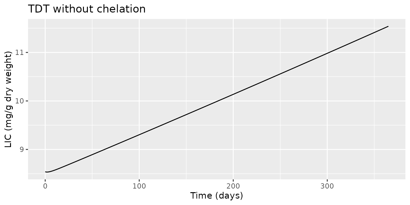
Verification datasets (Table S5)
Each Table S5 dataset is simulated with its own regimen, baseline LIC and transfusional iron loading (Table S1). Body weight comes from the Table S2 population equations at the midpoint of the dataset’s age range, weighted by the female fraction for the Thai datasets. Following the paper, each scenario is run for 30 days and LIC is extrapolated linearly to 6 or 12 months. The full-duration simulation is shown alongside.
wt_cauc <- function(age) {
  ht <- 156.00 + 0.2669 * age - 0.0072 * age^2
  exp(4.0279 - 0.0004 * ht)
}
wt_thai <- function(age, female) {
  ht_m <- 178.00 - 1.1936 * age + 0.0239 * age^2
  ht_f <- 148.31 + 0.3653 * age - 0.0037 * age^2
  (1 - female) * exp(3.9771 - 0.0003 * ht_m) + female * exp(3.7917 + 0.0003 * ht_f)
}
s5 <- tibble::tribble(
  ~dataset, ~pop, ~age_lo, ~age_hi, ~female, ~dose, ~lic_bl, ~transf, ~months, ~obs, ~paper_sim,
  10, "Caucasian", 18, 33, 0.75, 10, 8.77, 0.37, 6, 8.51, 7.64,
  11, "Caucasian", 19, 50, 0.58, 20, 8.54, 0.37, 6, 7.24, 7.08,
  20, "Thai", 23, 66, 0.67, 28, 14.86, 0.57, 6, 14.26, 11.90,
  21, "Thai", 18, 34, 0.13, 40, 29.44, 0.62, 6, 23.07, 22.79,
  14, "Caucasian", 18, 49, 0.53, 5, 2.5, 0.39, 12, 2.5 + 4.80, 2.5 + 1.69,
  15, "Caucasian", 18, 49, 0.53, 10, 4.9, 0.39, 12, 4.9 + 3.80, 4.9 - 0.39,
  16, "Caucasian", 18, 49, 0.53, 20, 10.6, 0.39, 12, 10.6 - 0.40, 10.6 - 3.95,
  17, "Caucasian", 18, 49, 0.53, 30, 24.2, 0.39, 12, 24.2 - 8.90, 24.2 - 11.45
) |>
  mutate(
    age = (age_lo + age_hi) / 2,
    WT = ifelse(pop == "Thai", wt_thai(age, female), wt_cauc(age)),
    id = seq_along(dataset)
  )

make_events <- function(d, days) {
  ev <- rxode2::et(
    amt = d$dose / mw_dfx * 1000, ii = 24, addl = days - 1, cmt = "gut"
  ) |>
    rxode2::et(seq(0, days * 24, by = 24)) |>
    as.data.frame()
  ev$id <- d$id
  ev$DIS_THALASSEMIA_TD <- 1
  ev$TRANSF_IRON_MGKGD <- d$transf
  ev$LIVER_IRON_BL <- d$lic_bl
  ev$WT <- d$WT
  ev
}
ev_s5 <- bind_rows(lapply(seq_len(nrow(s5)), function(i) make_events(s5[i, ], 365)))
sim_s5 <- rxode2::rxSolve(mod_drv, ev_s5, returnType = "data.frame", maxsteps = 1e6)
#> Warning: multi-subject simulation without without 'omega'

extrap <- sim_s5 |>
  filter(time <= 30 * 24) |>
  group_by(id) |>
  summarise(slope_per_day = coef(lm(liver_iron ~ I(time / 24)))[2], .groups = "drop")
full <- sim_s5 |>
  select(id, time, liver_iron)

s5_res <- s5 |>
  left_join(extrap, by = "id") |>
  mutate(
    end_day = months * 365 / 12,
    lic_extrap = lic_bl + slope_per_day * end_day
  ) |>
  rowwise() |>
  mutate(lic_full = full$liver_iron[full$id == id][which.min(abs(full$time[full$id == id] - end_day * 24))]) |>
  ungroup() |>
  mutate(pct_diff = 100 * (lic_extrap - paper_sim) / paper_sim)

s5_res |>
  select(dataset, months, dose, lic_bl, transf, WT, obs, paper_sim, lic_extrap, lic_full, pct_diff) |>
  mutate(across(c(WT, lic_extrap, lic_full, pct_diff), \(x) round(x, 2))) |>
  rename(
    "Dataset" = dataset, "Months" = months, "DFX (mg/kg/day)" = dose,
    "Baseline LIC" = lic_bl, "Transfusional iron (mg/kg/day)" = transf,
    "WT (kg)" = WT, "Observed LIC" = obs, "Paper simulated LIC" = paper_sim,
    "This model, 30-day extrapolation" = lic_extrap,
    "This model, full simulation" = lic_full, "% difference vs paper" = pct_diff
  ) |>
knitr::kable(caption = "Replicates Supplementary Table S5 of Sakares 2025 (LIC in mg/g).")| Dataset | Months | DFX (mg/kg/day) | Baseline LIC | Transfusional iron (mg/kg/day) | WT (kg) | Observed LIC | Paper simulated LIC | This model, 30-day extrapolation | This model, full simulation | % difference vs paper |
|---|---|---|---|---|---|---|---|---|---|---|
| 10 | 6 | 10 | 8.77 | 0.37 | 52.70 | 8.51 | 7.64 | 7.55 | 7.67 | -1.24 |
| 11 | 6 | 20 | 8.54 | 0.37 | 52.73 | 7.24 | 7.08 | 6.95 | 7.12 | -1.80 |
| 20 | 6 | 28 | 14.86 | 0.57 | 47.86 | 14.26 | 11.90 | 11.50 | 11.87 | -3.34 |
| 21 | 6 | 40 | 29.44 | 0.62 | 50.25 | 23.07 | 22.79 | 21.79 | 22.66 | -4.39 |
| 14 | 12 | 5 | 2.50 | 0.39 | 52.73 | 7.30 | 4.19 | 3.93 | 3.71 | -6.27 |
| 15 | 12 | 10 | 4.90 | 0.39 | 52.73 | 8.70 | 4.51 | 4.38 | 4.48 | -2.96 |
| 16 | 12 | 20 | 10.60 | 0.39 | 52.73 | 10.20 | 6.65 | 6.37 | 7.26 | -4.25 |
| 17 | 12 | 30 | 24.20 | 0.39 | 52.73 | 15.30 | 12.75 | 11.96 | 14.68 | -6.23 |
The 30-day extrapolation reproduces the paper’s simulated LIC closely across all eight datasets, even though the DFX driver is a one-compartment approximation of the paper’s PBPK output. The datasets 14-17 rows compare the 12-month LIC level (baseline plus the reported change).
Dose targeting (Figure 6 and Table S6)
The paper used the Thai TDT population (ages 18-60, equal sex) to predict LIC 6 months after starting DFX at 20, 30 or 40 mg/kg/day. The grid covers baseline LIC of 10-30 mg/g and transfusion regimens of 1-3 units every 3-4 weeks (Figure 6). The typical-value model is run over the same grid, using the paper’s 30-day extrapolation.
regimens <- tibble::tribble(
  ~regimen, ~transf,
  "1 unit / 4 wk", 0.16,
  "1 unit / 3 wk", 0.22,
  "2 units / 4 wk", 0.32,
  "2 units / 3 wk", 0.45,
  "3 units / 3 wk", 0.67
)
grid <- tidyr::expand_grid(lic_bl = c(10, 15, 22.5, 30), regimens, dose = c(20, 30, 40)) |>
  mutate(id = seq_len(n()), WT = wt_thai(39, 0.5))
ev_s6 <- bind_rows(lapply(seq_len(nrow(grid)), function(i) make_events(grid[i, ], 30)))
sim_s6 <- rxode2::rxSolve(mod_drv, ev_s6, returnType = "data.frame", maxsteps = 1e6)
#> Warning: multi-subject simulation without without 'omega'
res_s6 <- sim_s6 |>
  group_by(id) |>
  summarise(slope_per_day = coef(lm(liver_iron ~ I(time / 24)))[2], .groups = "drop") |>
  right_join(grid, by = "id") |>
  mutate(
    lic_6mo = lic_bl + slope_per_day * 365 / 2,
    reduction_pct = 100 * (1 - lic_6mo / lic_bl)
  )
The maintainers digitised the mean markers for the 20 and 30 mg/kg/day arms from Figure 6. The y position of each marker’s centroid (in pixels of the published 709 x 409 figure) is converted to LIC using the panel’s y-axis tick marks: five ticks spaced 16 px apart, with the lowest tick at 106, 194, 282 and 370 px for baseline LIC 10, 15, 22.5 and 30 mg/g. The tick intervals are 0.5, 0.75, 1.125 and 1.5 mg/g.
axis_cal <- tibble::tribble(
  ~lic_bl, ~y_low, ~tick_low, ~tick_step,
  10, 106, 7.5, 0.5,
  15, 194, 11.25, 0.75,
  22.5, 282, 16.875, 1.125,
  30, 370, 22.5, 1.5
)
fig6 <- tibble::tibble(
  lic_bl = rep(c(10, 15, 22.5, 30), each = 10),
  dose = rep(rep(c(20, 30), each = 5), 4),
  regimen = rep(regimens$regimen, 8),
  y_px = c(
    96.1, 93.1, 88.5, 82.6, 72.6, 98.4, 95.9, 92.1, 87.2, 78.9,
    188.8, 186.9, 183.1, 178.7, 169.0, 190.8, 189.0, 186.3, 182.4, 175.5,
    280.2, 278.6, 275.4, 271.4, 262.6, 282.2, 280.5, 278.2, 274.9, 269.0,
    369.1, 367.8, 364.6, 360.5, 352.9, 371.4, 370.5, 368.0, 364.9, 359.0
  )
) |>
  left_join(axis_cal, by = "lic_bl") |>
  mutate(paper_lic_6mo = tick_low + (y_low - y_px) / 16 * tick_step) |>
  select(lic_bl, dose, regimen, paper_lic_6mo)

fig6_cmp <- fig6 |>
  left_join(select(res_s6, lic_bl, dose, regimen, lic_6mo), by = c("lic_bl", "dose", "regimen")) |>
  mutate(pct_diff = 100 * (lic_6mo - paper_lic_6mo) / paper_lic_6mo)
fig6_cmp |>
  mutate(
    regimen = factor(regimen, levels = regimens$regimen),
    across(c(paper_lic_6mo, lic_6mo, pct_diff), \(x) round(x, 2))
  ) |>
  arrange(lic_bl, dose, regimen) |>
  rename(
    "Baseline LIC (mg/g)" = lic_bl, "DFX (mg/kg/day)" = dose,
    "Transfusion regimen" = regimen, "Figure 6 mean LIC" = paper_lic_6mo,
    "This model" = lic_6mo, "% difference" = pct_diff
  ) |>
knitr::kable(caption = "Replicates the 20 and 30 mg/kg/day means of Figure 6 of Sakares 2025 (LIC at 6 months, mg/g).")| Baseline LIC (mg/g) | DFX (mg/kg/day) | Transfusion regimen | Figure 6 mean LIC | This model | % difference |
|---|---|---|---|---|---|
| 10.0 | 20 | 1 unit / 4 wk | 7.81 | 7.76 | -0.60 |
| 10.0 | 20 | 1 unit / 3 wk | 7.90 | 7.84 | -0.82 |
| 10.0 | 20 | 2 units / 4 wk | 8.05 | 7.95 | -1.24 |
| 10.0 | 20 | 2 units / 3 wk | 8.23 | 8.07 | -2.00 |
| 10.0 | 20 | 3 units / 3 wk | 8.54 | 8.23 | -3.63 |
| 10.0 | 30 | 1 unit / 4 wk | 7.74 | 7.65 | -1.19 |
| 10.0 | 30 | 1 unit / 3 wk | 7.82 | 7.70 | -1.47 |
| 10.0 | 30 | 2 units / 4 wk | 7.93 | 7.78 | -1.93 |
| 10.0 | 30 | 2 units / 3 wk | 8.09 | 7.87 | -2.66 |
| 10.0 | 30 | 3 units / 3 wk | 8.35 | 8.00 | -4.16 |
| 15.0 | 20 | 1 unit / 4 wk | 11.49 | 11.39 | -0.88 |
| 15.0 | 20 | 1 unit / 3 wk | 11.58 | 11.47 | -0.96 |
| 15.0 | 20 | 2 units / 4 wk | 11.76 | 11.59 | -1.47 |
| 15.0 | 20 | 2 units / 3 wk | 11.97 | 11.72 | -2.05 |
| 15.0 | 20 | 3 units / 3 wk | 12.42 | 11.91 | -4.09 |
| 15.0 | 30 | 1 unit / 4 wk | 11.40 | 11.25 | -1.34 |
| 15.0 | 30 | 1 unit / 3 wk | 11.48 | 11.30 | -1.57 |
| 15.0 | 30 | 2 units / 4 wk | 11.61 | 11.39 | -1.90 |
| 15.0 | 30 | 2 units / 3 wk | 11.79 | 11.49 | -2.59 |
| 15.0 | 30 | 3 units / 3 wk | 12.12 | 11.63 | -4.00 |
| 22.5 | 20 | 1 unit / 4 wk | 17.00 | 16.81 | -1.13 |
| 22.5 | 20 | 1 unit / 3 wk | 17.11 | 16.89 | -1.28 |
| 22.5 | 20 | 2 units / 4 wk | 17.34 | 17.02 | -1.81 |
| 22.5 | 20 | 2 units / 3 wk | 17.62 | 17.18 | -2.51 |
| 22.5 | 20 | 3 units / 3 wk | 18.24 | 17.41 | -4.55 |
| 22.5 | 30 | 1 unit / 4 wk | 16.86 | 16.61 | -1.47 |
| 22.5 | 30 | 1 unit / 3 wk | 16.98 | 16.67 | -1.81 |
| 22.5 | 30 | 2 units / 4 wk | 17.14 | 16.77 | -2.18 |
| 22.5 | 30 | 2 units / 3 wk | 17.37 | 16.88 | -2.85 |
| 22.5 | 30 | 3 units / 3 wk | 17.79 | 17.05 | -4.16 |
| 30.0 | 20 | 1 unit / 4 wk | 22.58 | 22.23 | -1.57 |
| 30.0 | 20 | 1 unit / 3 wk | 22.71 | 22.32 | -1.68 |
| 30.0 | 20 | 2 units / 4 wk | 23.01 | 22.47 | -2.34 |
| 30.0 | 20 | 2 units / 3 wk | 23.39 | 22.64 | -3.19 |
| 30.0 | 20 | 3 units / 3 wk | 24.10 | 22.91 | -4.93 |
| 30.0 | 30 | 1 unit / 4 wk | 22.37 | 21.97 | -1.76 |
| 30.0 | 30 | 1 unit / 3 wk | 22.45 | 22.04 | -1.83 |
| 30.0 | 30 | 2 units / 4 wk | 22.69 | 22.15 | -2.39 |
| 30.0 | 30 | 2 units / 3 wk | 22.98 | 22.27 | -3.08 |
| 30.0 | 30 | 3 units / 3 wk | 23.53 | 22.46 | -4.53 |
summary(fig6_cmp$pct_diff)
#>    Min. 1st Qu.  Median    Mean 3rd Qu.    Max.
#> -4.9338 -2.9040 -1.9151 -2.2906 -1.4692 -0.6012
stopifnot(
  # Centre: a wrong flux or conversion shifts every cell by far more.
  abs(median(fig6_cmp$pct_diff)) < 5,
  quantile(abs(fig6_cmp$pct_diff), 0.9) < 6
)
The typical-value model sits on or slightly below the paper’s population means. The gap widens with transfusion burden, to about 5% at 3 units every 3 weeks. Two things in the paper raise its means there and are absent from a single typical subject driven by a fixed DFX profile. First, chelation depletes DFX more when more transfused iron is available (the Eq. 5 feedback). Second, the means average over a virtual population of varying body weight.
res_s6 |>
  mutate(regimen = factor(regimen, levels = regimens$regimen)) |>
  ggplot(aes(regimen, lic_6mo, colour = factor(dose))) +
  geom_point(position = position_dodge(width = 0.5)) +
  geom_point(
    data = mutate(fig6, regimen = factor(regimen, levels = regimens$regimen)),
    aes(y = paper_lic_6mo), shape = 4, position = position_dodge(width = 0.5)
  ) +
  geom_hline(aes(yintercept = 0.75 * lic_bl), linetype = 2) +
  facet_wrap(~lic_bl, scales = "free_y", labeller = label_both) +
  labs(
    x = "Transfusion regimen", y = "LIC at 6 months (mg/g)", colour = "DFX (mg/kg/day)",
    caption = "Dots: this model. Crosses: digitised Figure 6 means. Dashed line: 25% reduction target."
  ) +
  theme(axis.text.x = element_text(angle = 30, hjust = 1))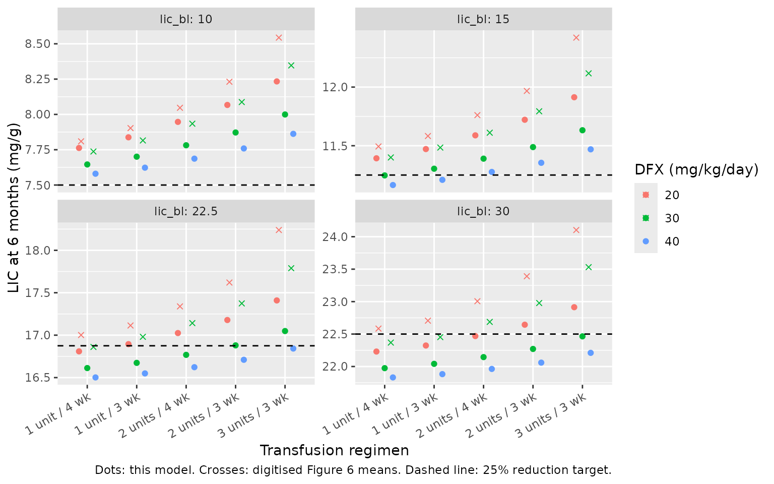
Replicates Figure 6 of Sakares 2025 (typical values only).
The targeted doses in Table S6 do not follow from the Figure 6 means. At a baseline LIC of 10 mg/g, for example, no mean reaches the 25% reduction target, in the paper or here, yet Table S6 lists 30-40 mg/kg/day for the lighter transfusion regimens. The table reads the lower end of the 5th-95th percentile band of the paper’s virtual trials instead. That band comes from Simcyp population variability, which the deterministic packaged model does not carry. Table S6 is therefore reproduced as reference, with this model’s typical-value percentage reduction at each dose:
paper_s6 <- tibble::tribble(
  ~lic_bl, ~regimen, ~paper_dose,
  10, "1 unit / 4 wk", "30", 10, "1 unit / 3 wk", "30", 10, "2 units / 4 wk", "40",
  10, "2 units / 3 wk", "N.A.", 10, "3 units / 3 wk", "N.A.",
  15, "1 unit / 4 wk", "20", 15, "1 unit / 3 wk", "20", 15, "2 units / 4 wk", "20",
  15, "2 units / 3 wk", "30", 15, "3 units / 3 wk", "40",
  22.5, "1 unit / 4 wk", "20", 22.5, "1 unit / 3 wk", "20", 22.5, "2 units / 4 wk", "20",
  22.5, "2 units / 3 wk", "20", 22.5, "3 units / 3 wk", "30",
  30, "1 unit / 4 wk", "20", 30, "1 unit / 3 wk", "20", 30, "2 units / 4 wk", "20",
  30, "2 units / 3 wk", "20", 30, "3 units / 3 wk", "20"
)
res_s6 |>
  select(lic_bl, regimen, dose, reduction_pct) |>
  mutate(dose = paste0("Reduction at ", dose, " mg/kg/day (%)"), reduction_pct = round(reduction_pct, 1)) |>
  tidyr::pivot_wider(names_from = dose, values_from = reduction_pct) |>
  left_join(paper_s6, by = c("lic_bl", "regimen")) |>
  mutate(regimen = factor(regimen, levels = regimens$regimen)) |>
  arrange(lic_bl, regimen) |>
  rename(
    "Baseline LIC (mg/g)" = lic_bl, "Transfusion regimen" = regimen,
    "Targeted dose, Table S6 (mg/kg/day)" = paper_dose
  ) |>
knitr::kable(caption = "Supplementary Table S6 of Sakares 2025 beside this model's typical-value 6-month LIC reduction.")| Baseline LIC (mg/g) | Transfusion regimen | Reduction at 20 mg/kg/day (%) | Reduction at 30 mg/kg/day (%) | Reduction at 40 mg/kg/day (%) | Targeted dose, Table S6 (mg/kg/day) |
|---|---|---|---|---|---|
| 10.0 | 1 unit / 4 wk | 22.4 | 23.5 | 24.2 | 30 |
| 10.0 | 1 unit / 3 wk | 21.6 | 23.0 | 23.8 | 30 |
| 10.0 | 2 units / 4 wk | 20.5 | 22.2 | 23.1 | 40 |
| 10.0 | 2 units / 3 wk | 19.3 | 21.3 | 22.4 | N.A. |
| 10.0 | 3 units / 3 wk | 17.7 | 20.0 | 21.4 | N.A. |
| 15.0 | 1 unit / 4 wk | 24.0 | 25.0 | 25.6 | 20 |
| 15.0 | 1 unit / 3 wk | 23.5 | 24.6 | 25.3 | 20 |
| 15.0 | 2 units / 4 wk | 22.7 | 24.1 | 24.8 | 20 |
| 15.0 | 2 units / 3 wk | 21.9 | 23.4 | 24.3 | 30 |
| 15.0 | 3 units / 3 wk | 20.6 | 22.5 | 23.5 | 40 |
| 22.5 | 1 unit / 4 wk | 25.3 | 26.2 | 26.7 | 20 |
| 22.5 | 1 unit / 3 wk | 24.9 | 25.9 | 26.4 | 20 |
| 22.5 | 2 units / 4 wk | 24.3 | 25.5 | 26.1 | 20 |
| 22.5 | 2 units / 3 wk | 23.7 | 25.0 | 25.7 | 20 |
| 22.5 | 3 units / 3 wk | 22.6 | 24.2 | 25.1 | 30 |
| 30.0 | 1 unit / 4 wk | 25.9 | 26.8 | 27.2 | 20 |
| 30.0 | 1 unit / 3 wk | 25.6 | 26.5 | 27.1 | 20 |
| 30.0 | 2 units / 4 wk | 25.1 | 26.2 | 26.8 | 20 |
| 30.0 | 2 units / 3 wk | 24.5 | 25.8 | 26.5 | 20 |
| 30.0 | 3 units / 3 wk | 23.6 | 25.1 | 26.0 | 20 |
The ordering is the paper’s. The reduction grows with baseline LIC and with dose, and shrinks as transfusion burden rises. That is why Table S6 asks for higher doses at low baseline LIC and heavy transfusion.
Assumptions and deviations
-
PK layer not reproduced. The DFX PBPK model is a
Simcyp V22 whole-body model (ADAM absorption, retrograde CYP1A2, CYP2D6
and biliary intrinsic clearances, Kp scalar 0.84) whose physiology and
tissue partitioning come from the simulator’s libraries and are not
printed. Only the iron PD layer is packaged. Users supply total plasma
DFX as
CP_DEFERASIROX_UM. In the paper, chelation also depletes DFX (Eq. 5); that feedback lives in the PBPK layer, and a supplied concentration that was measured or simulated after chelation already carries it. - Transfusional iron input. Table 1 lists the transfusional input k_blood (umol/L/h) only as “Various”, and Tables S1 and S6 give it in mg/kg/day. The model converts with the iron atomic mass (55.845 g/mol) and the chelatable-iron volume (5.40 L), so the conversion needs body weight. The paper does not print the weights it used. This vignette takes them from the Table S2 population equations. The Table S5 replication above (all eight datasets within a few percent of the paper’s simulated LIC) supports the conversion.
- Initial chelatable iron. Table 1 gives the initial chelatable iron only as “depending on the initial storage iron concentration” (Barry 1974). The model starts at 2.2853 umol/L, the healthy steady state of Eq. 1-2 at the Table 1 values. In TDT the starting value does not matter: chelation clears the pool within hours. Starting values from 0 to 300 umol/L change the 6-month LIC by less than 0.03%.
-
Equation 5. As typeset, Eq. 5 subtracts the
dissociation term
koff * complexfrom DFX rather than adding it back. It is not encoded here, because the DFX state belongs to the PBPK layer. -
Fixed versus estimated. The paper calibrated the PD
layer by hand and with COPASI rather than by population estimation.
Values the paper takes from the literature are wrapped in
fixed(). Values it estimated (uptake and efflux Vmax, efflux Km, the linear uptake constant) or tuned by hand (kon,keli) are not. -
No variability. The paper reports no
inter-individual variability or residual error for the PD layer;
between-subject variation in its simulations comes from the Simcyp
virtual population. The packaged model is deterministic
(
addSdfixed at 0). - Figure 6 and Table S6. The paper’s Figure 6 shows means and 5th-95th percentiles over 10 virtual trials of 10 subjects, and Table S6 reads its targeted doses from the lower percentile. This vignette uses one typical subject (age 39, Table S2 weight averaged over the sexes) and the one-compartment DFX driver. The packaged model reproduces the Figure 6 means but cannot give the percentiles, so it does not regenerate the Table S6 dose choices.
- Dataset 20 dose. Table S1 lists 30 mg/kg/day and Table S5 lists 28 mg/kg/day. The vignette uses Table S5, which reports the LIC result.