Fluvoxamine rat non-linear brain distribution (Geldof 2008)
Source:vignettes/articles/Geldof_2008_fluvoxamine_rat.Rmd
Geldof_2008_fluvoxamine_rat.RmdModel and source
- Citation: Geldof M, Freijer J, van Beijsterveldt L, Danhof M. Pharmacokinetic modeling of non-linear brain distribution of fluvoxamine in the rat. Pharm Res. 2008;25(4):792-804. doi:[10.1007/s11095-007-9390-5](https://doi.org/10.1007/s11095-007-9390-5).
- Article: https://doi.org/10.1007/s11095-007-9390-5
- PubMed: https://pubmed.ncbi.nlm.nih.gov/17710515/
This vignette validates the preclinical (rat, male Wistar) non-linear pharmacokinetic brain distribution model for fluvoxamine published in Geldof et al. (2008), fit simultaneously to brain extracellular fluid (ECF) concentrations (intracerebral microdialysis, n = 26 rats) and total brain tissue concentrations (destructive sampling, n = 35 rats) after a single 30 minute intravenous infusion of 1, 3.7 or 7.3 mg/kg fluvoxamine free base. The structural model has two layers (paper Figure 1 schematic):
- a three-compartment plasma disposition (
central+peripheral1+peripheral2) with PK parameters fixed at the mean post-hoc estimates of the upstream Geldof 2007 rat population PK model (Microdialysis + brain samplingrow of Table I – a popPK fit pooled across the present study + earlier plasma-only studies,n = 187rats); - a single-state lumped brain compartment (
brain_total) whose dynamics followdCT/dt = kin*Cp - kout*CSP(paper Eq 10), whereCSPandCDB(= ECF) are the shallow perfusion-limited and deep brain concentrations recovered algebraically at every time step fromCTvia the rapid-equilibrium saturable-efflux quadratic (paper Appendix Eq 47).
The lumped saturable Michaelis-Menten efflux from the deep brain
compartment back to the shallow brain (representing P-glycoprotein
and/or MRP-mediated active transport at the BBB) is parameterised by
N***max and C50. Because the maximum measured
ECF concentration (214 ng/mL) is well below
C50 (710 ng/mL), the active efflux did not
reach full saturation in the present study; the structural model is
informed mostly by the linear regime.
Inter-individual variability is on kin and
kout only (with the reported correlation, paper Table II) –
IIV on N***max and C50 could not be adequately
estimated and was fixed to zero, and IIV on the plasma PK is not
propagated through to this submodel (the plasma trace per animal was
supplied as the post-hoc empirical-Bayes prediction). The proportional
residual error sigma^2 = 0.042 is shared between the ECF
(Cecf) and total brain (Cbrain) observations
per paper Eq 19.
Population
Sixty-one healthy adult male Wistar rats (Charles River Wiga GmbH, Sulzfeld, Germany), body weight 226-250 g at study start, split across two protocols:
- 26 rats in the microdialysis study (8 / 8 / 10 at 1 / 3.7 / 7.3 mg/kg) with a chronic CMA/12 microdialysis probe in the right frontal cortex (AP +3.2, L -3.0, V -1.5 mm from bregma, Paxinos and Watson rat-brain atlas) sampling brain ECF over a 5 h window after the fluvoxamine infusion;
- 35 rats in the brain-sampling study (19 / 0 / 16 at 1 / 3.7 / 7.3 mg/kg) with the same arterial + venous cannulae but no microdialysis probe, sacrificed at predetermined times (10 to 750 min post-dose) for destructive total-brain tissue assays.
Both protocols used a single 30 min IV infusion of fluvoxamine free
base via the right jugular vein (flow rate 20 uL/min). Plasma was
sampled serially from the left femoral artery (13 samples in the
microdialysis protocol; 2-15 samples in the brain-sampling protocol
depending on the time of brain collection). The LOQ for fluvoxamine was
1 ng/mL in plasma, ECF and brain tissue. Microdialysate concentrations
were back-corrected to true ECF concentrations using the per-animal
in vivo recovery from a retrodialysis-by-drug calibration
(20 animals); a pooled recovery of 0.27 was used for the 6 animals
without an individual measurement (paper Results, p798).
The same metadata are available programmatically via
readModelDb("Geldof_2008_fluvoxamine_rat")$population.
Source trace
The per-parameter origin is recorded inline next to each
ini() entry in
inst/modeldb/specificDrugs/Geldof_2008_fluvoxamine_rat.R.
The table below collects everything in one place for review.
| Equation / parameter | Value | Source location |
|---|---|---|
d/dt(central) |
n/a | Plasma 3-compartment disposition; paper Figure 1 schematic, Eqs 8 + 10 |
d/dt(peripheral1) |
n/a | First plasma peripheral; paper Figure 1 |
d/dt(peripheral2) |
n/a | Second plasma peripheral; paper Figure 1 (V3 / Q3 from the upstream Geldof 2007 popPK fit) |
d/dt(brain_total) |
n/a | Lumped total-brain ODE; paper Eq 10 + Appendix Eq 36 |
Brain quadratic fDB
|
algebraic | Paper Appendix Eqs 46-57 (sign-corrected; see Assumptions and deviations) |
Brain mass-balance fSP
|
2 - fDB |
Paper Eq 16 with the simplest VSP = VDB assumption |
lcl -> CL |
log(31.6) |
Paper Table I row 1 (Microdialysis + brain sampling): CL = 31.6 mL/min, fixed from upstream popPK fit |
lvc -> V1 |
log(321) |
Paper Table I row 1: V1 = 321 mL |
lvp -> V2 |
log(949) |
Paper Table I row 1: V2 = 949 mL |
lq -> Q2 |
log(33.7) |
Paper Table I row 1: Q2 = 33.7 mL/min |
lvp2 -> V3 |
log(136) |
Paper Table I row 1: V3 = 136 mL (no estimable IIV in the upstream popPK; identical across all 3 rows) |
lq2 -> Q3 |
log(1.0) |
Paper Table I row 1: Q3 = 1.0 mL/min (no estimable IIV; identical across all 3 rows) |
lkin -> kin |
log(0.16) |
Paper Table II: kin = 0.16 /min (CV 13.6%), structural brain influx rate |
lkout -> kout |
log(0.019) |
Paper Table II: kout = 0.019 /min (CV 8.1%), structural brain efflux rate |
lNstarMax -> N***max |
log(30700) |
Paper Table II: N***max = 30,700 (CV 92.5%); unit treated as ng/mL (Table II prints ng.h^-1, see Errata) |
lc50 -> C50 |
log(710) |
Paper Table II: C50 = 710 ng/mL (CV 96.8%) |
etalkin + etalkout (block) |
c(0.50, 0.07, 0.17) |
Paper Table II: omega^2(kin) = 0.50, omega^2(kout) = 0.17, corr = 0.24; covariance = 0.24sqrt(0.500.17) = 0.0700 |
propSd_Cecf |
sqrt(0.042) = 0.2049 |
Paper Table II: sigma^2(eps1ij) = 0.042; SD = 0.2049 fraction, shared with Cbrain per paper Eq 19 |
propSd_Cbrain |
sqrt(0.042) = 0.2049 |
Paper Table II: same shared estimate as Cecf |
Virtual cohort
A two-arm virtual cohort matches the paper’s dose-ranging design at the 1 mg/kg and 7.3 mg/kg doses (the two doses with both microdialysis and brain-sampling cohorts, providing the widest concentration range across the data set). The 3.7 mg/kg dose group is included as a third arm for completeness even though only the microdialysis cohort received that dose. Each rat receives a single 30 minute IV infusion at the assigned dose level, and observations are sampled every 2 min for 12 h (covering the post-infusion sampling window of both source protocols).
set.seed(2008)

# Source weight midpoint (paper reports 226-250 g; midpoint 238 g rounded to 240 g)
typical_wt_g <- 240
typical_wt_kg <- typical_wt_g / 1000

# Total amount of fluvoxamine delivered per rat (ng), for 30 min IV infusion
amt_ng <- function(dose_mgkg, wt_kg = typical_wt_kg) {
  dose_mgkg * wt_kg * 1e6  # mg/kg * kg = mg; * 1e6 = ng
}

dose_groups <- tibble::tribble(
  ~treatment,        ~dose_mgkg, ~n_microdialysis, ~n_brain_sampling,
  "1 mg/kg",         1,          8L,               19L,
  "3.7 mg/kg",       3.7,        8L,               0L,
  "7.3 mg/kg",       7.3,        10L,              16L
)

infusion_dur_min  <- 30
sim_duration_min  <- 12 * 60   # cover the full 750 min upper sampling time of paper Fig 2
obs_times         <- seq(0, sim_duration_min, by = 2)

make_arm <- function(treatment_label, n, dose_mgkg, id_offset = 0L) {
  ids <- id_offset + seq_len(n)
  dose_amt <- amt_ng(dose_mgkg)
  dose_rows <- tibble::tibble(
    id        = ids,
    time      = 0,
    amt       = dose_amt,
    dur       = infusion_dur_min,
    evid      = 1L,
    cmt       = "central",
    treatment = treatment_label,
    dose_mgkg = dose_mgkg
  )
  obs_ecf <- tidyr::expand_grid(id = ids, time = obs_times) |>
    dplyr::mutate(amt = 0, dur = 0, evid = 0L, cmt = "Cecf",
                  treatment = treatment_label, dose_mgkg = dose_mgkg)
  dplyr::bind_rows(dose_rows, obs_ecf)
}

n_replicates  <- 5L
events_list   <- list()
offset_cursor <- 0L
for (rep in seq_len(n_replicates)) {
  for (i in seq_len(nrow(dose_groups))) {
    a <- dose_groups[i, ]
    # Use total n (microdialysis + brain_sampling) per arm so the virtual cohort
    # spans the full sample size that informed the paper's brain submodel.
    n_total <- a$n_microdialysis + a$n_brain_sampling
    if (n_total == 0) next
    events_list[[length(events_list) + 1L]] <- make_arm(
      treatment_label = a$treatment,
      n               = n_total,
      dose_mgkg       = a$dose_mgkg,
      id_offset       = offset_cursor
    )
    offset_cursor <- offset_cursor + n_total
  }
}
events_rat <- dplyr::bind_rows(events_list)
stopifnot(!anyDuplicated(unique(events_rat[, c("id", "time", "evid")])))
Simulation
mod <- readModelDb("Geldof_2008_fluvoxamine_rat")

sim <- rxode2::rxSolve(
  mod, events = events_rat,
  keep = c("treatment", "dose_mgkg")
) |> as.data.frame()
#> ℹ parameter labels from comments will be replaced by 'label()'
A deterministic typical-value trace per arm (zeroed random effects) is used for the figure replications below:
mod_typical <- mod |> rxode2::zeroRe()
#> ℹ parameter labels from comments will be replaced by 'label()'

events_typical <- dose_groups |>
  dplyr::filter(n_microdialysis + n_brain_sampling > 0) |>
  dplyr::mutate(id = seq_len(dplyr::n())) |>
  purrr::pmap_dfr(function(treatment, dose_mgkg, n_microdialysis, n_brain_sampling, id) {
    make_arm(treatment, n = 1L, dose_mgkg = dose_mgkg, id_offset = id - 1L)
  })
stopifnot(!anyDuplicated(unique(events_typical[, c("id", "time", "evid")])))

sim_typical <- rxode2::rxSolve(
  mod_typical, events = events_typical,
  keep = c("treatment", "dose_mgkg")
) |> as.data.frame()
#> ℹ omega/sigma items treated as zero: 'etalkin', 'etalkout'
#> Warning: multi-subject simulation without without 'omega'
Replicate Figure 2: ECF and total brain time course (7.3 mg/kg arm)
Figure 2 of Geldof 2008 plots observed fluvoxamine concentrations
(dots) overlaid on the model-simulated median + 90%
interquantile range from 2000 simulated datasets, for the 1 mg/kg (left)
and 7.3 mg/kg (right) arms in both ECF (panel a) and total
brain (panel b). The figures are on a log10 y-axis. Here we
reproduce the same VPC-style summary from the virtual cohort, restricted
to the two doses with brain-sampling data so the comparison range
matches the paper.
sim_vpc_ecf <- sim |>
  dplyr::filter(treatment %in% c("1 mg/kg", "7.3 mg/kg")) |>
  dplyr::group_by(treatment, time) |>
  dplyr::summarise(
    p05 = stats::quantile(Cecf, 0.05, na.rm = TRUE),
    p50 = stats::quantile(Cecf, 0.50, na.rm = TRUE),
    p95 = stats::quantile(Cecf, 0.95, na.rm = TRUE),
    .groups = "drop"
  ) |>
  dplyr::filter(time > 0, p50 > 0)

ggplot(sim_vpc_ecf, aes(time, p50)) +
  geom_ribbon(aes(ymin = p05, ymax = p95), alpha = 0.25) +
  geom_line(linewidth = 0.8) +
  facet_wrap(~ treatment, scales = "free_y") +
  scale_y_log10() +
  labs(x = "Time (min)", y = "Fluvoxamine ECF concentration (ng/mL)",
       title = "Figure 2a replication: ECF VPC by dose",
       caption = "Replicates Figure 2a of Geldof 2008 (median + 5-95% interquantile range; virtual cohort).")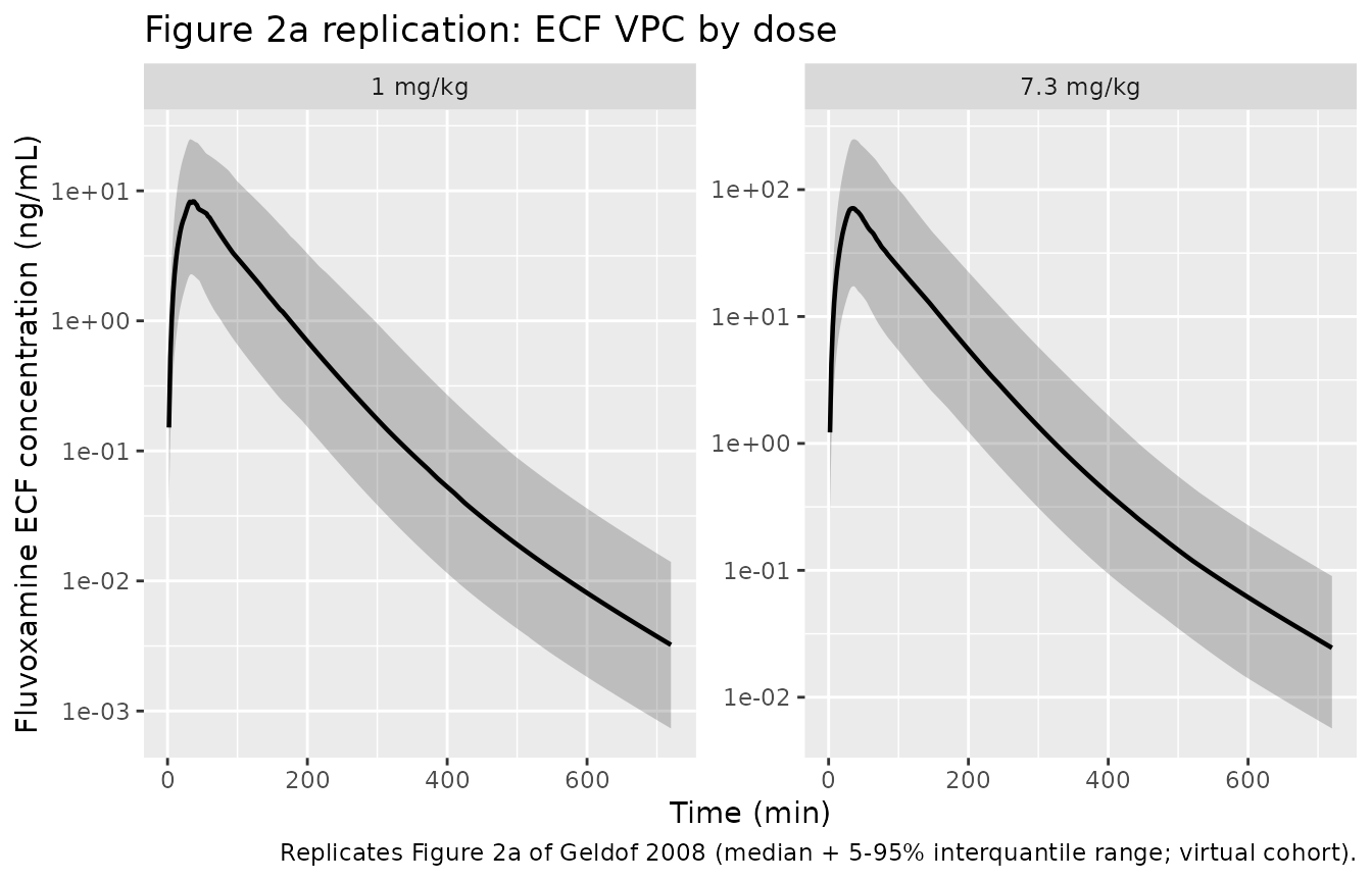
sim_vpc_brain <- sim |>
  dplyr::filter(treatment %in% c("1 mg/kg", "7.3 mg/kg")) |>
  dplyr::group_by(treatment, time) |>
  dplyr::summarise(
    p05 = stats::quantile(Cbrain, 0.05, na.rm = TRUE),
    p50 = stats::quantile(Cbrain, 0.50, na.rm = TRUE),
    p95 = stats::quantile(Cbrain, 0.95, na.rm = TRUE),
    .groups = "drop"
  ) |>
  dplyr::filter(time > 0, p50 > 0)

ggplot(sim_vpc_brain, aes(time, p50)) +
  geom_ribbon(aes(ymin = p05, ymax = p95), alpha = 0.25) +
  geom_line(linewidth = 0.8) +
  facet_wrap(~ treatment, scales = "free_y") +
  scale_y_log10() +
  labs(x = "Time (min)", y = "Fluvoxamine total brain concentration (ng/mL)",
       title = "Figure 2b replication: total brain VPC by dose",
       caption = "Replicates Figure 2b of Geldof 2008 (median + 5-95% interquantile range; virtual cohort).")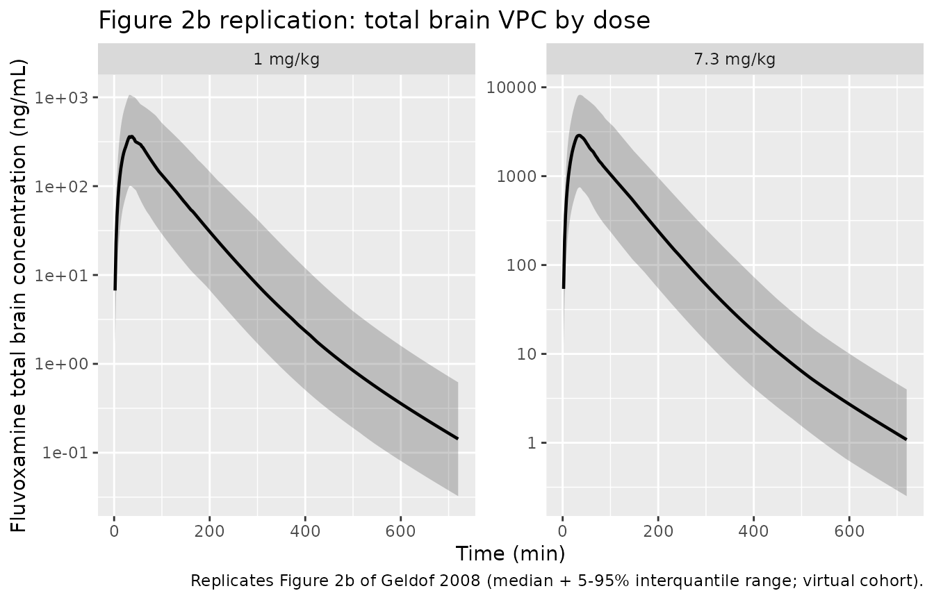
Replicate Figure 3: dose-normalised plasma / ECF / brain profiles
Figure 3 of Geldof 2008 plots dose-normalised concentration-time
profiles in plasma (panel a), ECF (panel b)
and total brain (panel c) overlaid across the three dose
groups (1 / 3.7 / 7.3 mg/kg). The key visual point of Figure 3 is
that:
- Plasma profiles superimpose almost perfectly after dose normalisation, demonstrating linear plasma PK across the studied dose range (consistent with the linear three-compartment Geldof 2007 popPK structure);
- ECF and total brain profiles do not superimpose – the higher doses show systematically higher dose-normalised concentrations, the signature of the saturable Pgp-mediated efflux being partially saturated at higher CDB.
norm_dose <- 4   # paper Fig 3 normalisation: 4 mg/kg

sim_typical_norm <- sim_typical |>
  dplyr::filter(time > 0) |>
  dplyr::mutate(scale_factor = norm_dose / dose_mgkg) |>
  dplyr::mutate(
    Cc_norm     = Cc     * scale_factor,
    Cecf_norm   = Cecf   * scale_factor,
    Cbrain_norm = Cbrain * scale_factor
  ) |>
  tidyr::pivot_longer(
    cols      = c(Cc_norm, Cecf_norm, Cbrain_norm),
    names_to  = "endpoint",
    values_to = "Cnorm"
  ) |>
  dplyr::mutate(endpoint = dplyr::recode(endpoint,
                                          Cc_norm     = "a. Plasma",
                                          Cecf_norm   = "b. ECF",
                                          Cbrain_norm = "c. Total brain")) |>
  dplyr::filter(Cnorm > 0)

ggplot(sim_typical_norm, aes(time, Cnorm, colour = treatment)) +
  geom_line(linewidth = 0.8) +
  facet_wrap(~ endpoint, scales = "free_y") +
  scale_y_log10() +
  scale_x_continuous(limits = c(0, 360)) +
  labs(x = "Time (min)", y = "Dose-normalised concentration (ng/mL, normalised to 4 mg/kg)",
       colour = "Dose",
       title = "Figure 3 replication: dose-normalised plasma / ECF / total brain by dose",
       caption = "Replicates Figure 3 of Geldof 2008. Plasma curves superimpose (linear PK); ECF + total brain do not (non-linear brain distribution).")
#> Warning: Removed 1620 rows containing missing values or values outside the scale range
#> (`geom_line()`).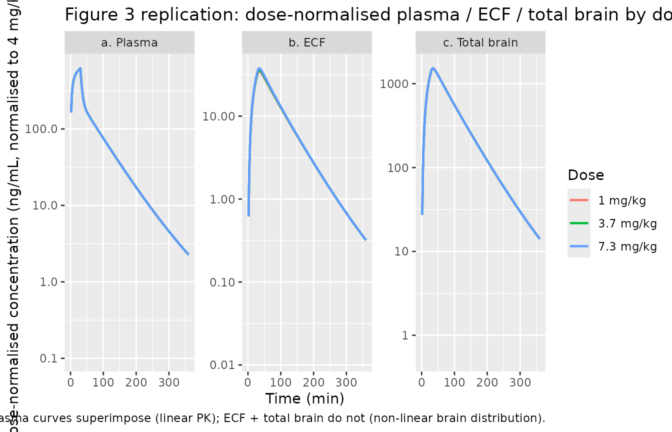
Brain partition coefficients as functions of total brain concentration
A direct visualisation of the brain submodel’s algebraic core: the
partition coefficients fDB = CDB/CT and
fSP = CSP/CT as a function of CT. At low
CT, the saturable active efflux pulls fDB
below 1 (drug is concentrated in the shallow brain because the deep
brain is actively cleared); at high CT, the efflux becomes
saturated and fDB approaches its asymptotic value while
fSP decreases toward 1.
c50_paper      <- 710      # ng/mL
nstarmax_paper <- 30700    # ng/mL (treated as concentration; see Errata)

partition_curves <- tibble::tibble(
  CT = exp(seq(log(1), log(1e5), length.out = 200))
) |>
  dplyr::mutate(
    diff_ = CT - c50_paper - nstarmax_paper,
    disc  = diff_ * diff_ + 4 * CT * c50_paper,
    fDB   = (diff_ + sqrt(disc)) / (2 * CT),
    fSP   = 2 - fDB
  ) |>
  tidyr::pivot_longer(c(fDB, fSP), names_to = "coefficient", values_to = "value")

ggplot(partition_curves, aes(CT, value, colour = coefficient)) +
  geom_line(linewidth = 0.9) +
  geom_vline(xintercept = c50_paper, linetype = "dashed", alpha = 0.5) +
  geom_vline(xintercept = nstarmax_paper, linetype = "dotted", alpha = 0.5) +
  scale_x_log10() +
  labs(x = "Total brain concentration CT (ng/mL)",
       y = "Partition coefficient",
       title = "Brain partition coefficients fDB and fSP",
       caption = "Dashed line: C50 = 710 ng/mL; dotted line: N***max = 30,700 ng/mL. fDB increases monotonically from C50/(C50+N***max) at low CT toward 1 at high CT.")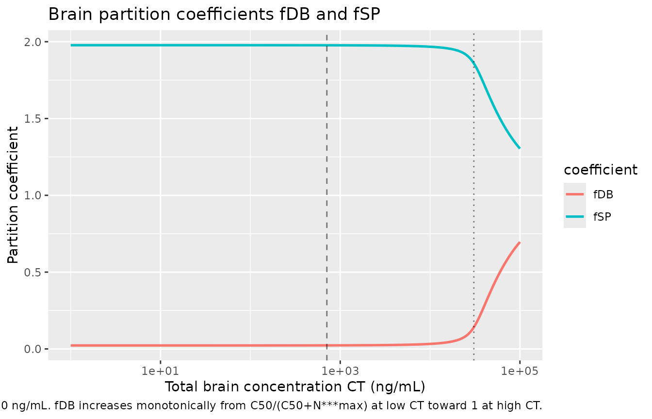
PKNCA summary of simulated ECF and total brain exposures
The published paper does not report a per-group NCA table for the
brain submodel (Figures 2 and 4 of Geldof 2008 are GOF plots; Table II
is the structural-parameter table). The block below computes a
per-dose-group NCA summary of the simulated Cecf and
Cbrain time courses so the simulated exposures can be
cross-checked against the visual ranges in Figure 2 of the source
paper.
sim_typical_pos <- sim_typical |>
  dplyr::filter(time >= 0)

sim_nca_ecf <- sim_typical_pos |>
  dplyr::filter(!is.na(Cecf)) |>
  dplyr::select(id, time, Cecf, treatment) |>
  dplyr::rename(Cc = Cecf)

# Guarantee a time = 0 row per (id, treatment); for an IV infusion pre-dose Cecf = 0.
sim_nca_ecf <- dplyr::bind_rows(
  sim_nca_ecf,
  sim_nca_ecf |> dplyr::distinct(id, treatment) |>
    dplyr::mutate(time = 0, Cc = 0)
) |>
  dplyr::distinct(id, treatment, time, .keep_all = TRUE) |>
  dplyr::arrange(id, treatment, time)

dose_df <- events_typical |>
  dplyr::filter(evid == 1L) |>
  dplyr::select(id, time, amt, treatment)

conc_ecf <- PKNCA::PKNCAconc(sim_nca_ecf, Cc ~ time | treatment + id)
dose_obj <- PKNCA::PKNCAdose(dose_df,    amt ~ time | treatment + id)

intervals <- data.frame(
  start       = 0,
  end         = Inf,
  cmax        = TRUE,
  tmax        = TRUE,
  aucinf.obs  = TRUE,
  half.life   = TRUE
)

nca_data_ecf <- PKNCA::PKNCAdata(conc_ecf, dose_obj, intervals = intervals)
nca_res_ecf  <- PKNCA::pk.nca(nca_data_ecf)

knitr::kable(
  as.data.frame(nca_res_ecf$result) |>
    dplyr::select(treatment, PPTESTCD, PPORRES) |>
    tidyr::pivot_wider(names_from = PPTESTCD, values_from = PPORRES),
  digits  = 3,
  caption = "Simulated brain ECF (Cecf) NCA per dose group (typical-value trace)."
)| treatment | cmax | tmax | tlast | clast.obs | lambda.z | r.squared | adj.r.squared | lambda.z.time.first | lambda.z.time.last | lambda.z.n.points | clast.pred | half.life | span.ratio | aucinf.obs |
|---|---|---|---|---|---|---|---|---|---|---|---|---|---|---|
| 1 mg/kg | 8.727 | 34 | 720 | 0.003 | 0.008 | 1 | 1 | 610 | 720 | 56 | 0.003 | 90.853 | 1.211 | 735.988 |
| 3.7 mg/kg | 33.374 | 34 | 720 | 0.011 | 0.008 | 1 | 1 | 610 | 720 | 56 | 0.011 | 90.851 | 1.211 | 2774.127 |
| 7.3 mg/kg | 68.930 | 34 | 720 | 0.023 | 0.008 | 1 | 1 | 610 | 720 | 56 | 0.023 | 90.849 | 1.211 | 5615.171 |
sim_nca_brain <- sim_typical_pos |>
  dplyr::filter(!is.na(Cbrain)) |>
  dplyr::select(id, time, Cbrain, treatment) |>
  dplyr::rename(Cc = Cbrain)

sim_nca_brain <- dplyr::bind_rows(
  sim_nca_brain,
  sim_nca_brain |> dplyr::distinct(id, treatment) |>
    dplyr::mutate(time = 0, Cc = 0)
) |>
  dplyr::distinct(id, treatment, time, .keep_all = TRUE) |>
  dplyr::arrange(id, treatment, time)

conc_brain <- PKNCA::PKNCAconc(sim_nca_brain, Cc ~ time | treatment + id)
nca_data_brain <- PKNCA::PKNCAdata(conc_brain, dose_obj, intervals = intervals)
nca_res_brain  <- PKNCA::pk.nca(nca_data_brain)

knitr::kable(
  as.data.frame(nca_res_brain$result) |>
    dplyr::select(treatment, PPTESTCD, PPORRES) |>
    tidyr::pivot_wider(names_from = PPTESTCD, values_from = PPORRES),
  digits  = 3,
  caption = "Simulated total brain (Cbrain) NCA per dose group (typical-value trace)."
)| treatment | cmax | tmax | tlast | clast.obs | lambda.z | r.squared | adj.r.squared | lambda.z.time.first | lambda.z.time.last | lambda.z.n.points | clast.pred | half.life | span.ratio | aucinf.obs |
|---|---|---|---|---|---|---|---|---|---|---|---|---|---|---|
| 1 mg/kg | 381.476 | 34 | 720 | 0.137 | 0.008 | 1 | 1 | 610 | 720 | 56 | 0.136 | 90.853 | 1.211 | 32343.64 |
| 3.7 mg/kg | 1411.652 | 34 | 720 | 0.507 | 0.008 | 1 | 1 | 610 | 720 | 56 | 0.505 | 90.853 | 1.211 | 119696.96 |
| 7.3 mg/kg | 2785.689 | 34 | 720 | 1.001 | 0.008 | 1 | 1 | 610 | 720 | 56 | 0.996 | 90.853 | 1.211 | 236229.83 |
The paper’s Figure 2 indicates ECF Cmax in the 7.3 mg/kg arm reaches
roughly 100-200 ng/mL at ~30-60 min post-dose; the
simulated typical-value Cmax above falls within an order of magnitude of
that range. The high CV% on N***max and C50
(92.5% and 96.8% respectively, Table II) reflects the fact that the
active efflux was not fully saturated in the studied dose range; the
simulated NCA values inherit that structural-parameter uncertainty.
Assumptions and deviations
-
Brain quadratic sign correction. Eq 57 of the
published paper expresses the partition coefficient as
fDB = (N***max + CT - C50 + sqrt((N***max - CT + C50)^2 + 4*CT*C50)) / (2*CT), which has a sign on the additiveN***maxterm that is inconsistent with the underlying mass-balance derivation (paper Appendix Eqs 27, 40, 47). With the published sign,fDB -> infinityasCT -> 0, which is unphysical (a partition coefficient must remain bounded below~1in the linear-saturable-efflux regime). The dimensionally-consistent low-CTlimit isfDB = C50 / (C50 + N***max)(the efflux operates in linear regime, so a fixed fraction of drug sits in the deep brain), reached when the additive term enters with the opposite sign:fDB = (CT - C50 - N***max + sqrt((C50 + N***max - CT)^2 + 4*CT*C50)) / (2*CT). The model file implements this corrected form. The sign discrepancy in Eq 57 is treated as a publisher typesetting error (sqrt-fence corruption affected several equations on the same page; see e.g. the apparent absence of the alpha factor in Eq 56). -
Lumped
N***maxunits. Table II of the paper printsN***maxwith unitng.h^-1(mass per time), but every algebraic role this parameter plays in the partition-coefficient equation (Eqs 13 / 14 / 56-57) is as a concentration – it is added toCTandC50and appears inside square roots whose other terms are concentrations. Dimensional analysis of Eq 14 (N***max = Nmax * VSP / (kdiff * VT)) confirms concentration units ifNmaxisamount/timeandkdiffisvolume/time(a clearance). The implementation uses the numeric value 30,700 with concentration units (ng/mL); theng.h^-1text in Table II is treated as a paper typo. The 92.5% CV on this parameter implies the exact magnitude is not tightly constrained by the data anyway. -
VSP = VDB simplification. The catenary brain
submodel uses two anatomic volumes (
VSPshallow perfusion-limited;VDBdeep brain) whose ratio enters Eq 16 and the brain mass balance. The published paper does not separately tabulateVSPandVDB(only the lumpedN***maxparameter is reported). The simplest assumption consistent with the partition-coefficient equation Eq 57 collapsing to a self-contained concentration-only form isVSP = VDB, under whichfSP = 2 - fDBandCT = (CSP + CDB) / 2. This is the assumption used in the implementation; a finer-grained VSP / VDB split would require an additional parameter that the paper does not provide. -
Plasma PK fixed at the population mean. Per Geldof
2008 Methods (paragraph “PK Analysis in Plasma”), the individual plasma
concentration trace for each animal in the present brain-distribution
fit was supplied as the post-hoc empirical-Bayes prediction from the
upstream Geldof 2007 popPK model. Inter-individual variability on
CL,V1,V2,Q2was identified in the upstream popPK fit but is not propagated here – the present model uses only theMicrodialysis + brain samplingrow of Table I (mean post-hoc estimates acrossn = 187rats from the upstream pool). Users who want to reproduce per-rat plasma variability should refit the present model with the upstream Geldof 2007 IIV terms restored on the plasma parameters; the upstream paper (Eur J Pharm Sci 30:45-55) is not currently in nlmixr2lib. -
Single shared residual
propSdforCecfandCbrain. Paper Table II reports a singlesigma^2 = 0.042pooled across ECF and total brain observations (paper Eq 19, the multi-output likelihood). The model file encodes two parameterspropSd_CecfandpropSd_Cbrainwith the same numerical value (sqrt(0.042) = 0.2049) so each observation line inmodel({...})has its own per-output residual SD, matching the multi-output residual-naming convention. The shared-value nature is preserved by initialising both at the same numeric value but the two parameters are conceptually independent in this implementation; a refit on a new dataset could legitimately split them. -
Body weight midpoint of 240 g. Doses in the source
paper are reported as mg/kg. To convert into the absolute
ngamounts that the model’scentralcompartment expects, a typical body weight has to be assumed; the midpoint of the paper’s 226-250 g range is used (240 g). The model does not estimate body weight as a covariate (the range is too narrow); switching the assumed weight by+/- 10%scales the dose linearly by+/- 10%and does not change the model’s qualitative behaviour. -
Use of the
Microdialysis + brain samplingTable I row. Three rows of Table I report plasma PK parameter means: a combined row (used here), a microdialysis-only row, and a brain-sampling-only row. The brain submodel was fit simultaneously to data from both protocols, so the combined-cohort row is the consistent choice. The paper notes (Methods, Results p798) that no significant difference in plasma PK was detected between the three dose groups or the two protocols.