Fruquintinib concentration-QTc (Zhou 2025)
Source:vignettes/articles/Zhou_2025_fruquintinib.Rmd
Zhou_2025_fruquintinib.RmdModel and source
- Citation: Zhou X, Toms A, Morton D, Wang X, Taylor A, Dasari A, Gupta N, Chien C. Assessment of the Effects of Fruquintinib on Cardiac Safety in Patients with Metastatic Colorectal Cancer. The Journal of Clinical Pharmacology 2025;65(11):1411-1419. doi:10.1002/jcph.70051.
- Article: https://doi.org/10.1002/jcph.70051
Zhou et al. (2025) report the cardiac-safety analysis of fruquintinib, a highly selective oral inhibitor of vascular endothelial growth factor receptors 1, 2 and 3 approved for previously treated metastatic colorectal cancer (mCRC). The analysis uses concentration-QTc (C-QTc) modelling on the ECG substudy of the phase 3 FRESCO-2 trial (NCT04322539), in which patients received fruquintinib 5 mg once daily – or matching placebo – on days 1-21 of a 28-day cycle.
The paper fits linear mixed-effects models of the change from baseline in the corrected QT interval against time-matched plasma concentrations, following the methods of Garnett et al. and ICH E14. Three model families were estimated (parent fruquintinib only, metabolite M11 only, and both together) on two heart-rate corrections, and three of the resulting fits are reported with full parameter tables. Per the standing “replicate the author’s structure” policy, each is packaged as its own model file, all pointing at this one vignette:
| Model file | Endpoint | Driver | Role in the paper | Source table |
|---|---|---|---|---|
Zhou_2025_fruquintinib_QTcP_M11 |
DeltaQTcP | M11 | Final model (lowest AIC, 10727.07) | Table 2 |
Zhou_2025_fruquintinib_QTcF_M11 |
DeltaQTcF | M11 | Supportive analysis | Suppl. Table 4 |
Zhou_2025_fruquintinib_QTcP_parent |
DeltaQTcP | fruquintinib | Additional analysis (negative result) | Suppl. Table 5 |
Two features of the paper drive the encoding and are worth stating up front.
QTcP, not QTcF, is the primary endpoint. A graphical
assessment showed Fridericia’s formula did not adequately correct heart
rate in this cohort: the baseline QTcF-RR slope was 0.0493 (90% CI
0.0393, 0.0592), statistically significant, whereas the population-based
correction gave a QTcP-RR slope of -3.73e-05 with a 90% CI (-0.0102,
0.0101) spanning zero. QTcP is the population-based correction
QTcP = QT / RR^beta, with beta estimated from
a log-log regression of QT on RR fitted to the cohort’s cycle 1 day 1
pre-dose replicates. The QTcF fit is reported as a supportive analysis
for cross-comparison with conventional thorough-QT analyses.
The models are PD-only. No population PK model is
fitted anywhere in the source, so both plasma concentrations are
consumed as time-varying covariates
(CP_FRUQUINTINIB_M11_NGML and
CP_FRUQUINTINIB_NGML, both ng/mL). A user who wants a full
DeltaQTc time course from a dose record must therefore supply the
concentration trajectory from a separate PK model.
Zhou_2025_fruquintinib_poppk (the companion population PK
analysis by the same first author, doi:10.1002/jcph.70001,
validated in vignette("Zhou_2025_fruquintinib_poppk"))
supplies exactly that: it returns Cc and
Cc_m11 in ng/mL, the units these models expect. Note that
the two analyses were fitted independently on different datasets – the
C-QTc models here use the FRESCO-2 ECG substudy, whereas the popPK model
pools six studies – so pairing them is a reasonable simulation workflow,
not a joint fit the authors performed.
model_names <- c(
  "Zhou_2025_fruquintinib_QTcP_M11",
  "Zhou_2025_fruquintinib_QTcF_M11",
  "Zhou_2025_fruquintinib_QTcP_parent"
)
# Resolve each to an rxUi exactly once; readModelDb() returns the model
# FUNCTION, not a ui, and downstream accessors need the ui.
uis <- lapply(model_names, function(n) rxode2::rxode(readModelDb(n)))
names(uis) <- model_names
stopifnot(all(vapply(uis, function(u) inherits(u, "rxUi"), logical(1))))
Population
The C-QTc analysis set comprises 1456 time-matched concentration-DeltaQTcP pairs from 205 patients with previously treated mCRC – 137 in the fruquintinib arm and 68 in the placebo arm. These were drawn from 1954 sets of Holter ECG measurements in 243 patients (163 fruquintinib, 80 placebo); records were excluded for missing baseline QTc, for ECG measurements without a time-matched concentration, and where ECG and PK sampling were performed more than 30 minutes apart.
Twelve-lead ECGs were extracted in triplicate from continuous Holter recordings and processed centrally by eResearch Technology, Inc. The trial excluded patients with a QTcF > 480 ms, patients with any other factor that could prolong the QTc interval or increase arrhythmic risk, and patients receiving concomitant QTc-prolonging medication; such comedications were prohibited on study. The mean baseline QTcP and QTcF in the analysis set were 419.3 ms and 409.5 ms respectively – these are the two centering references used by the model files.
Of the 936 fruquintinib-arm concentration pairs, 16 (1.7%) fruquintinib concentrations and 326 (34.8%) M11 concentrations were below the limit of quantification; BLQ values were set to zero and retained in the analysis. All placebo records were assigned a concentration of 0 at every nominal time point. The high M11 BLQ fraction is precisely why the authors also ran the parent-driven analysis as a cross-check.
The same information is available programmatically via each model’s
population metadata, e.g.
rxode2::rxode(readModelDb("Zhou_2025_fruquintinib_QTcP_M11"))$population.
Source trace
The per-parameter origin is recorded as an in-file comment next to
each ini() entry. The table below collects them in one
place for review. Every value is transcribed from a published point
estimate; none is derived, digitised, or carried from another
publication.
| Model | Parameter | Value | Source location |
|---|---|---|---|
| QTcP/M11 | e0 |
2.82 ms | Table 2 ‘Intercept’ (SE 1.35; P = 0.0372) |
| QTcP/M11 | e_on_treatment_e0 |
-5.19 ms | Table 2 ‘Treatment’ (SE 1.36; P = 0.0002) |
| QTcP/M11 | slope |
0.0339 ms/(ng/mL) | Table 2 ‘M11 conc. slope’ (SE 0.0147; P = 0.0212) |
| QTcP/M11 |
e_ntime1_e0 .. e_ntime4_e0
|
-0.25, 1.78, 1.84, 0.570 ms | Table 2 ‘NTime = 1’ .. ‘NTime = 4’ |
| QTcP/M11 | e_day21_e0 |
-1.39 ms | Table 2 ‘Cycle 1 day 21 visit’ (SE 0.676; P = 0.0406) |
| QTcP/M11 | e_qtc_bl_e0 |
-0.102 ms/ms | Table 2 ‘Baseline QTcP’ (SE 0.0306; P = 0.0011) |
| QTcP/M11 | etae0 |
8.23^2 = 67.7329 | Table 2 ‘BSV SD for intercept’ = 8.23 ms |
| QTcP/M11 | etaslope |
0.0953^2 = 0.00908209 | Table 2 ‘BSV SD of the M11 conc. slope’ = 0.0953 |
| QTcP/M11 | addSd |
7.93 ms | Table 2 ‘Residual error SD’ (SE 0.165) |
| QTcP/M11 | qtc_bl_ref |
419.3 ms | Results, ‘Summary of Data Used for Analysis’ |
| QTcF/M11 | e0 |
2.37 ms | Suppl. Table 4 ‘Intercept’ (SE 1.31; P = 0.0695) |
| QTcF/M11 | e_on_treatment_e0 |
-3.34 ms | Suppl. Table 4 ‘Treatment’ (SE 1.32; P = 0.0122) |
| QTcF/M11 | slope |
0.0477 ms/(ng/mL) | Suppl. Table 4 ‘M11 Conc. Slope’ (SE 0.0163; P = 0.0035) |
| QTcF/M11 |
e_ntime1_e0 .. e_ntime4_e0
|
0.964, 2.73, 2.69, 1.42 ms | Suppl. Table 4 ‘NTime=1’ .. ‘NTime=4’ |
| QTcF/M11 | e_day21_e0 |
-1.50 ms | Suppl. Table 4 ‘Cycle 1 Day 21 Visit’ (SE 0.652) |
| QTcF/M11 | e_qtc_bl_e0 |
-0.118 ms/ms | Suppl. Table 4 ‘Baseline QTcF’ (SE 0.0286) |
| QTcF/M11 | etae0 |
8.02^2 = 64.3204 | Suppl. Table 4 ‘BSV SD for Intercept’ = 8.02 ms |
| QTcF/M11 | etaslope |
0.116^2 = 0.013456 | Suppl. Table 4 ‘BSV SD of Conc. Slope’ = 0.116 |
| QTcF/M11 | addSd |
7.54 ms | Suppl. Table 4 ‘Residual Error SD’ (SE 0.157) |
| QTcF/M11 | qtc_bl_ref |
409.5 ms | Results, ‘Summary of Data Used for Analysis’ |
| QTcP/parent | e0 |
2.33 ms | Suppl. Table 5 ‘Intercept’ (SE 1.31; P = 0.0756) |
| QTcP/parent | e_on_treatment_e0 |
-5.24 ms | Suppl. Table 5 ‘Treatment’ (SE 1.46; P = 0.0004) |
| QTcP/parent | slope |
0.00778 ms/(ng/mL) | Suppl. Table 5 ‘Fruquintinib Conc. Slope’ (P = 0.1377) |
| QTcP/parent |
e_ntime1_e0 .. e_ntime4_e0
|
-0.254, 1.6, 1.6, 0.353 ms | Suppl. Table 5 ‘NTime=1’ .. ‘NTime=4’ |
| QTcP/parent | e_qtc_bl_e0 |
-0.105 ms/ms | Suppl. Table 5 ‘Baseline QTcP’ (SE 0.0309) |
| QTcP/parent |
etae0 + etaslope block |
74.3044 / -0.117232 / 0.0016 | Suppl. Table 5 SDs 8.62 and 0.0400 with correlation -0.340 |
| QTcP/parent | addSd |
8.02 ms | Suppl. Table 5 ‘Residual Error SD’ (SE 0.167) |
| QTcP/parent | (no visit term) | dropped | Suppl. Table 1, model fit.f.2 (LRT P = 0.1318) |
Transcription audit
The source tables report, for every row, an estimate, its standard
error, a relative standard error, and a 95% confidence interval. Those
four quantities are algebraically redundant, which makes them a
mechanical check on the transcription:
RSE% = 100 * SE / |estimate| must reproduce the printed
RSE, and the printed interval must bracket the printed estimate. A
dropped minus sign, a transposed digit, or a row read off the wrong
table breaks at least one of the two relations.
This matters more than usual here. The main-text PDF renders negative
numbers with a space after the minus sign (- 5.19), so sign
errors are a live risk, and three of the four coefficients that a naive
automated source-trace check failed to find in the paper were negative
for exactly that reason. The audit below reads the estimates back out of
the built models – not out of a hand-written list – so it also confirms
that what reached ini() is what the tables print.
# Published SE / RSE% / 95% CI, transcribed alongside each ini() parameter.
published <- tibble::tribble(
  ~model,        ~param,              ~se,      ~rse,   ~lo,      ~hi,
  "QTcP_M11",    "e0",                1.35,     47.9,    0.176,    5.47,
  "QTcP_M11",    "e_on_treatment_e0", 1.36,     26.2,   -7.86,    -2.52,
  "QTcP_M11",    "slope",             0.0147,   43.4,    0.00516,  0.0625,
  "QTcP_M11",    "e_ntime1_e0",       0.867,   347,     -1.95,     1.45,
  "QTcP_M11",    "e_ntime2_e0",       0.867,    48.7,    0.0873,   3.48,
  "QTcP_M11",    "e_ntime3_e0",       0.868,    47.2,    0.144,    3.54,
  "QTcP_M11",    "e_ntime4_e0",       0.874,   153,     -1.14,     2.28,
  "QTcP_M11",    "e_day21_e0",        0.676,    48.6,   -2.71,    -0.0638,
  "QTcP_M11",    "e_qtc_bl_e0",       0.0306,   30.0,   -0.162,   -0.0415,
  "QTcP_M11",    "addSd",             0.165,     2.08,   7.61,     8.26,
  "QTcF_M11",    "e0",                1.31,     55.3,   -0.182,    4.93,
  "QTcF_M11",    "e_on_treatment_e0", 1.32,     39.5,   -5.94,    -0.743,
  "QTcF_M11",    "slope",             0.0163,   34.2,    0.0158,   0.0795,
  "QTcF_M11",    "e_ntime1_e0",       0.826,    85.7,   -0.651,    2.58,
  "QTcF_M11",    "e_ntime2_e0",       0.826,    30.3,    1.12,     4.35,
  "QTcF_M11",    "e_ntime3_e0",       0.826,    30.7,    1.07,     4.31,
  "QTcF_M11",    "e_ntime4_e0",       0.833,    58.7,   -0.210,    3.05,
  "QTcF_M11",    "e_day21_e0",        0.652,    43.5,   -2.78,    -0.226,
  "QTcF_M11",    "e_qtc_bl_e0",       0.0286,   24.2,   -0.174,   -0.0621,
  "QTcF_M11",    "addSd",             0.157,     2.08,   7.24,     7.86,
  "QTcP_parent", "e0",                1.31,     56.2,   -0.233,    4.89,
  "QTcP_parent", "e_on_treatment_e0", 1.46,     27.9,   -8.12,    -2.37,
  "QTcP_parent", "slope",             0.00524,  67.4,   -0.00247,  0.018,
  "QTcP_parent", "e_ntime1_e0",       0.851,   335,     -1.92,     1.41,
  "QTcP_parent", "e_ntime2_e0",       0.846,    52.9,   -0.0524,   3.26,
  "QTcP_parent", "e_ntime3_e0",       0.846,    52.9,   -0.0611,   3.25,
  "QTcP_parent", "e_ntime4_e0",       0.854,   242,     -1.32,     2.02,
  "QTcP_parent", "e_qtc_bl_e0",       0.0309,   29.4,   -0.166,   -0.0442,
  "QTcP_parent", "addSd",             0.167,     2.08,   7.70,     8.35
)

# Pull the point estimates back out of the BUILT models.
fitted_theta <- lapply(model_names, function(n) {
  d <- uis[[n]]$iniDf
  d <- d[is.na(d$neta1), c("name", "est")]
  d$model <- sub("^Zhou_2025_fruquintinib_", "", n)
  d
}) |> dplyr::bind_rows()

audit <- published |>
  dplyr::left_join(fitted_theta, by = c("model", "param" = "name")) |>
  dplyr::mutate(
    rse_calc = 100 * se / abs(est),
    rse_ok   = abs(rse_calc - rse) <= pmax(0.5, 0.005 * rse),
    ci_ok    = est >= lo & est <= hi,
    wald_z   = ((hi - lo) / 2) / se,
    wald_ok  = abs(wald_z - 1.96) < 0.25
  )

# Guard the guard: a join that matched nothing would make every all() vacuous.
stopifnot(
  nrow(audit) == nrow(published),
  !anyNA(audit$est),
  all(audit$rse_ok),
  all(audit$ci_ok),
  all(audit$wald_ok)
)

audit |>
  dplyr::summarise(
    .by = model,
    `Rows audited`            = dplyr::n(),
    `Max RSE% discrepancy`    = max(abs(rse_calc - rse)),
    `Estimate inside 95% CI`  = all(ci_ok),
    `Wald z (min)`            = min(wald_z),
    `Wald z (max)`            = max(wald_z)
  ) |>
  dplyr::rename("Model" = model) |>
  knitr::kable(
    digits = 3,
    caption = paste(
      "Transcription audit. For every fixed-effect and residual-error",
      "parameter, the recomputed RSE% reproduces the printed RSE% and the",
      "printed 95% CI brackets the estimate that reached ini(). The implied",
      "Wald multiplier sits at 1.96 throughout, confirming these are",
      "symmetric 95% normal-theory intervals."
    )
)| Model | Rows audited | Max RSE% discrepancy | Estimate inside 95% CI | Wald z (min) | Wald z (max) |
|---|---|---|---|---|---|
| QTcP_M11 | 10 | 0.333 | TRUE | 1.950 | 1.970 |
| QTcF_M11 | 10 | 0.044 | TRUE | 1.951 | 1.975 |
| QTcP_parent | 9 | 0.074 | TRUE | 1.946 | 1.971 |
The between-subject variability and correlation rows are audited
separately, because ini() stores variances and a covariance
while the tables print standard deviations and a correlation.
bsv_published <- tibble::tribble(
  ~model,        ~quantity,      ~sd_or_cor, ~se,      ~rse,  ~lo,     ~hi,
  "QTcP_M11",    "SD intercept",  8.23,      0.486,     5.91,  7.33,    9.24,
  "QTcP_M11",    "SD slope",      0.0953,    0.0118,   12.4,   0.0751,  0.121,
  "QTcF_M11",    "SD intercept",  8.02,      0.473,     5.90,  7.14,    9.00,
  "QTcF_M11",    "SD slope",      0.116,     0.013,    11.2,   0.0938,  0.145,
  "QTcP_parent", "SD intercept",  8.62,      0.591,     6.86,  7.54,    9.85,
  "QTcP_parent", "SD slope",      0.0400,    0.00485,  12.1,   0.0316,  0.0505,
  "QTcP_parent", "Correlation",  -0.340,     0.141,    41.5,  -0.551,  -0.0872
)

stopifnot(
  nrow(bsv_published) == 7L,
  all(abs(100 * bsv_published$se / abs(bsv_published$sd_or_cor) -
            bsv_published$rse) <= pmax(0.5, 0.005 * bsv_published$rse)),
  all(bsv_published$sd_or_cor >= bsv_published$lo &
        bsv_published$sd_or_cor <= bsv_published$hi)
)

# The omega entries that reached ini(), and what they should be.
omega_expected <- tibble::tribble(
  ~model,        ~entry,               ~expected,
  "QTcP_M11",    "etae0",               8.23^2,
  "QTcP_M11",    "etaslope",            0.0953^2,
  "QTcF_M11",    "etae0",               8.02^2,
  "QTcF_M11",    "etaslope",            0.116^2,
  "QTcP_parent", "etae0",               8.62^2,
  "QTcP_parent", "etaslope",            0.0400^2,
  "QTcP_parent", "(etae0,etaslope)",   -0.340 * 8.62 * 0.0400
)

omega_fitted <- lapply(model_names, function(n) {
  d <- uis[[n]]$iniDf
  d <- d[!is.na(d$neta1), c("name", "est")]
  d$model <- sub("^Zhou_2025_fruquintinib_", "", n)
  d
}) |> dplyr::bind_rows()

omega_chk <- omega_expected |>
  dplyr::left_join(omega_fitted, by = c("model", "entry" = "name"))
stopifnot(
  nrow(omega_chk) == 7L,
  !anyNA(omega_chk$est),
  all(abs(omega_chk$est - omega_chk$expected) < 1e-9)
)

omega_chk |>
  dplyr::mutate(`Abs. difference` = abs(est - expected)) |>
  dplyr::rename(
    "Model"                     = model,
    "ini() entry"               = entry,
    "Expected (from published)" = expected,
    "In model file"             = est
  ) |>
  knitr::kable(
    digits = 8,
    caption = paste(
      "Between-subject variability audit. Every omega entry in ini() equals",
      "the square of the published SD (or, for the parent model's",
      "off-diagonal, correlation x SD x SD) exactly."
    )
)| Model | ini() entry | Expected (from published) | In model file | Abs. difference |
|---|---|---|---|---|
| QTcP_M11 | etae0 | 67.73290000 | 67.73290000 | 0 |
| QTcP_M11 | etaslope | 0.00908209 | 0.00908209 | 0 |
| QTcF_M11 | etae0 | 64.32040000 | 64.32040000 | 0 |
| QTcF_M11 | etaslope | 0.01345600 | 0.01345600 | 0 |
| QTcP_parent | etae0 | 74.30440000 | 74.30440000 | 0 |
| QTcP_parent | etaslope | 0.00160000 | 0.00160000 | 0 |
| QTcP_parent | (etae0,etaslope) | -0.11723200 | -0.11723200 | 0 |
The parent model’s 2x2 block must also be a valid covariance matrix;
a correlation encoded with the wrong sign or magnitude would show up as
an indefinite matrix and rxSolve would fail with
chol(): decomposition failed.
om <- matrix(c(8.62^2, -0.340 * 8.62 * 0.0400,
               -0.340 * 8.62 * 0.0400, 0.0400^2), 2, 2)
eig <- eigen(om, symmetric = TRUE, only.values = TRUE)$values
stopifnot(all(eig > 0), det(om) > 0)
cat(sprintf("determinant = %.6f; eigenvalues = %.6f, %.6f\n",
            det(om), eig[1], eig[2]))
#> determinant = 0.105144; eigenvalues = 74.304585, 0.001415
Virtual cohort
The three models are purely algebraic – there is no ODE system and no time dependence in the PD expression, because the paper’s mixed-effects fit relates a single ECG reading to the concentration drawn at the same nominal time. A single event-table row per scenario is therefore sufficient; no time course needs to be integrated.
The covariate grid the paper actually sampled is the product of two
visits (cycle 1 day 1 and cycle 1 day 21) and five nominal times (0, 1,
2, 3, 4 h after dose), crossed with the two randomized arms.
NTIME carries the nominal hour and DAY21 the
visit; QTC_BL is set to the reported cohort mean so the
centered-baseline term collapses to zero and the model returns the
typical-baseline prediction.
# One observation event per scenario row. The models declare no ODE states, so
# cmt is NA_character_ -- there is no compartment to align an observation onto,
# and naming the observable here would be the slot-renumbering bug.
make_events <- function(df, conc_col) {
  stopifnot(nrow(df) > 0L, conc_col %in% names(df))
  out <- df
  out$id   <- seq_len(nrow(out))
  out$time <- 0
  out$evid <- 0
  out$amt  <- 0
  out$cmt  <- NA_character_
  out
}
Structural gate: the placebo-corrected contrast
The paper’s headline quantity is the placebo-corrected change from baseline, DeltaDeltaQTc. Its Methods define it as
mean DeltaDeltaQTc = mean(DeltaQTc | TRT = 1, C = C) - mean(DeltaQTc | TRT = 0, C = 0)Every term of the linear predictor except the treatment offset and
the concentration slope – the intercept, the nominal-time coefficients,
the visit coefficient, the centered-baseline term – is common to both
arms and cancels, so the contrast collapses to
e_on_treatment_e0 + slope * C. That is a structural claim
about the encoding, and it is worth testing as one rather than asserting
it: the check below forms the contrast by solving the model
twice and differencing, at every nominal time and both visits, and
requires the result to be invariant to those nuisance covariates.
solve_typical <- function(ui, ev) {
  as.data.frame(rxode2::rxSolve(rxode2::zeroRe(ui), events = ev))
}

# Full nuisance-covariate grid crossed with both arms, at the two published
# M11 scenarios.
grid_qtcp <- tidyr::expand_grid(
  conc         = c(77, 154),
  NTIME        = c(0, 1, 2, 3, 4),
  DAY21        = c(0, 1),
  ON_TREATMENT = c(0, 1)
) |>
  dplyr::mutate(
    QTC_BL = 419.3,
    # placebo records carry zero concentration by construction
    CP_FRUQUINTINIB_M11_NGML = dplyr::if_else(ON_TREATMENT == 1, conc, 0)
  )

grid_ev  <- make_events(grid_qtcp, "CP_FRUQUINTINIB_M11_NGML")
# Join the solve back onto the event table by id rather than binding by
# position, so a reordered solve cannot silently mislabel a covariate cell.
sim_grid <- solve_typical(
  uis[["Zhou_2025_fruquintinib_QTcP_M11"]], grid_ev
) |>
  dplyr::select(id, QTcP) |>
  dplyr::inner_join(
    grid_ev |> dplyr::select(id, conc, NTIME, DAY21, ON_TREATMENT),
    by = "id"
  )
#> ℹ omega/sigma items treated as zero: 'etae0', 'etaslope'
#> Warning: multi-subject simulation without without 'omega'
stopifnot(nrow(sim_grid) == nrow(grid_ev), !anyNA(sim_grid$QTcP))

contrast <- sim_grid |>
  tidyr::pivot_wider(
    id_cols     = c(conc, NTIME, DAY21),
    names_from  = ON_TREATMENT,
    values_from = QTcP,
    names_prefix = "arm"
  ) |>
  dplyr::mutate(ddqtcp = arm1 - arm0)

# The contrast must be identical across all 10 nuisance-covariate cells at
# each concentration -- that is the cancellation, tested rather than assumed.
spread_by_conc <- contrast |>
  dplyr::summarise(.by = conc, spread = max(ddqtcp) - min(ddqtcp), n = dplyr::n())
stopifnot(nrow(spread_by_conc) == 2L, all(spread_by_conc$n == 10L),
          all(spread_by_conc$spread < 1e-9))

knitr::kable(
  spread_by_conc |>
    dplyr::rename("M11 (ng/mL)" = conc,
                  "Range of DeltaDeltaQTcP across covariate cells (ms)" = spread,
                  "Cells" = n),
  digits = 12,
  caption = paste(
    "Cancellation gate: the placebo-corrected contrast is invariant to nominal",
    "time, visit and baseline across all 10 nuisance-covariate cells, to",
    "machine precision."
  )
)| M11 (ng/mL) | Range of DeltaDeltaQTcP across covariate cells (ms) | Cells |
|---|---|---|
| 77 | 0 | 10 |
| 154 | 0 | 10 |
Reproducing the published DeltaDeltaQTc predictions (Tables 3 and 4)
With the cancellation confirmed, the contrast can be compared directly against the paper’s own predictions at the geometric-mean steady-state M11 Cmax (77 ng/mL) and twice that value (154 ng/mL). These are the numbers the regulatory conclusion rests on.
ddqtc_at <- function(ui, obs_var, conc, conc_col, qtc_bl) {
  ev <- make_events(
    tibble::tibble(
      ON_TREATMENT = c(1, 0),
      NTIME        = 0,
      DAY21        = 1,
      QTC_BL       = qtc_bl,
      !!conc_col  := c(conc, 0)
    ),
    conc_col
  )
  s <- solve_typical(ui, ev)
  s[[obs_var]][1] - s[[obs_var]][2]
}

pred_tab <- tibble::tribble(
  ~endpoint, ~scenario,                          ~conc, ~paper,
  "QTcP",    "GM M11 Cmax at steady state",         77, -2.58,
  "QTcP",    "2 x GM M11 Cmax at steady state",    154,  0.0251,
  "QTcF",    "GM M11 Cmax at steady state",         77,  0.331,
  "QTcF",    "2 x GM M11 Cmax at steady state",    154,  4.00
) |>
  dplyr::rowwise() |>
  dplyr::mutate(
    model = if (endpoint == "QTcP") "Zhou_2025_fruquintinib_QTcP_M11"
            else "Zhou_2025_fruquintinib_QTcF_M11",
    qtc_bl = if (endpoint == "QTcP") 419.3 else 409.5,
    model_pred = ddqtc_at(uis[[model]], endpoint, conc,
                          "CP_FRUQUINTINIB_M11_NGML", qtc_bl),
    difference = model_pred - paper
  ) |>
  dplyr::ungroup()
#> ℹ omega/sigma items treated as zero: 'etae0', 'etaslope'
#> ℹ omega/sigma items treated as zero: 'etae0', 'etaslope'
#> ℹ omega/sigma items treated as zero: 'etae0', 'etaslope'
#> ℹ omega/sigma items treated as zero: 'etae0', 'etaslope'
#> Warning: There were 4 warnings in `dplyr::mutate()`.
#> The first warning was:
#> ℹ In argument: `model_pred = ddqtc_at(...)`.
#> ℹ In row 1.
#> Caused by warning:
#> ! multi-subject simulation without without 'omega'
#> ℹ Run `dplyr::last_dplyr_warnings()` to see the 3 remaining warnings.

# The paper prints its coefficients to 3 significant figures, so the
# reproduction error is bounded by propagated rounding of the two terms that
# survive the cancellation: half-ulp on the treatment offset (5e-3 ms) plus
# C times half-ulp on the slope (154 * 5e-5 = 7.7e-3 ms) -> ~1.3e-2 ms.
stopifnot(nrow(pred_tab) == 4L, max(abs(pred_tab$difference)) < 0.02)

pred_tab |>
  dplyr::select(endpoint, scenario, conc, paper, model_pred, difference) |>
  dplyr::rename(
    "Endpoint"                  = endpoint,
    "Scenario"                  = scenario,
    "M11 conc. (ng/mL)"         = conc,
    "Paper mean DeltaDelta (ms)" = paper,
    "Model mean DeltaDelta (ms)" = model_pred,
    "Difference (ms)"           = difference
  ) |>
  knitr::kable(
    digits = 4,
    caption = paste(
      "Replicates Table 3 (QTcP) and Table 4 (QTcF) of Zhou 2025. All four",
      "predictions reproduce to within 0.02 ms, the bound set by the paper's",
      "3-significant-figure coefficient rounding."
    )
)| Endpoint | Scenario | M11 conc. (ng/mL) | Paper mean DeltaDelta (ms) | Model mean DeltaDelta (ms) | Difference (ms) |
|---|---|---|---|---|---|
| QTcP | GM M11 Cmax at steady state | 77 | -2.5800 | -2.5797 | 0.0003 |
| QTcP | 2 x GM M11 Cmax at steady state | 154 | 0.0251 | 0.0306 | 0.0055 |
| QTcF | GM M11 Cmax at steady state | 77 | 0.3310 | 0.3329 | 0.0019 |
| QTcF | 2 x GM M11 Cmax at steady state | 154 | 4.0000 | 4.0058 | 0.0058 |
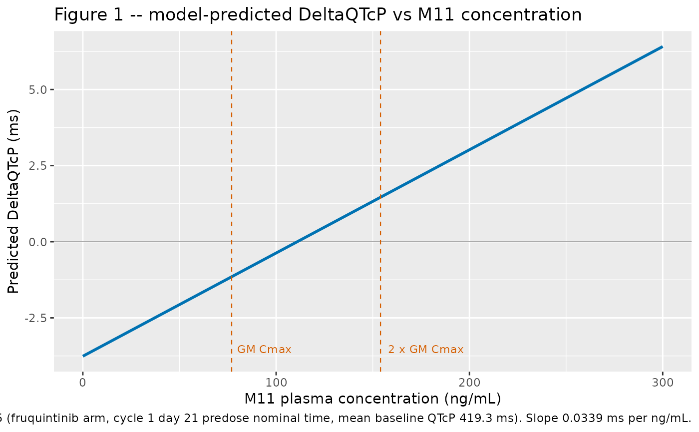
Replicate Figure 1
Figure 1 of the paper overlays the model-predicted DeltaQTcP on the
observed data as a function of M11 concentration. Its caption fixes the
covariate setting: “assuming a nominal time of cycle 1 day 21 predose
and a baseline QTcP equal to the mean value in the analysis dataset” –
i.e. NTIME = 0, DAY21 = 1,
QTC_BL = 419.3, on the fruquintinib arm (placebo records
carry M11 = 0 by construction, so the line over positive concentration
is the active arm).
fig1_grid <- tibble::tibble(
  CP_FRUQUINTINIB_M11_NGML = seq(0, 300, by = 2)
) |>
  dplyr::mutate(ON_TREATMENT = 1, NTIME = 0, DAY21 = 1, QTC_BL = 419.3)

fig1 <- solve_typical(
  uis[["Zhou_2025_fruquintinib_QTcP_M11"]],
  make_events(fig1_grid, "CP_FRUQUINTINIB_M11_NGML")
)
#> ℹ omega/sigma items treated as zero: 'etae0', 'etaslope'
#> Warning: multi-subject simulation without without 'omega'

ggplot(fig1, aes(CP_FRUQUINTINIB_M11_NGML, QTcP)) +
  geom_hline(yintercept = 0, linewidth = 0.3, colour = "grey60") +
  geom_line(linewidth = 1, colour = "#0072B2") +
  geom_vline(xintercept = c(77, 154), linetype = "dashed",
             colour = "#D55E00", linewidth = 0.4) +
  annotate("text", x = 77, y = min(fig1$QTcP), label = "GM Cmax",
           hjust = -0.1, vjust = -0.4, size = 3, colour = "#D55E00") +
  annotate("text", x = 154, y = min(fig1$QTcP), label = "2 x GM Cmax",
           hjust = -0.1, vjust = -0.4, size = 3, colour = "#D55E00") +
  labs(
    x = "M11 plasma concentration (ng/mL)",
    y = "Predicted DeltaQTcP (ms)",
    title = "Figure 1 -- model-predicted DeltaQTcP vs M11 concentration",
    caption = paste(
      "Replicates the model-prediction line of Figure 1 of Zhou 2025",
      "(fruquintinib arm, cycle 1 day 21 predose nominal time, mean baseline",
      "QTcP 419.3 ms). Slope 0.0339 ms per ng/mL."
    )
  )
Validation against observed summary statistics (Supplementary Table 6)
The gates so far test the contrast, which is a difference of two model predictions and therefore blind to the intercept, nominal-time and visit coefficients – exactly the terms that cancel. Supplementary Table 6 closes that gap. It reports the observed mean DeltaQTcP by treatment, visit and nominal time, and for the placebo arm the model prediction reduces to
DeltaQTcP = e0 + ntime_effect + e_day21_e0 * DAY21with no concentration term at all. Those nine cells therefore gate precisely the coefficients the contrast cannot see, against observed data, with no simulation and no seed.
The comparison is scaled by the standard error of each observed mean
(SD / sqrt(N), both published in the same table) rather
than expressed in raw milliseconds. A raw-ms bound would be arbitrary:
the observed placebo means carry roughly +/-1.5 ms of sampling noise in
their own right on 50-66 observations, so a 1 ms discrepancy is
meaningful at one cell and negligible at another. The standardized
residual is the quantity that is comparable across cells.
# Zhou 2025 Supplementary Table 6, placebo rows. Cycle 1 day 1 has no 0 h row
# because DeltaQTcP is identically zero at the pre-dose baseline reading.
obs_placebo <- tibble::tribble(
  ~DAY21, ~NTIME, ~n,  ~obs_mean, ~obs_sd,
       0,      1, 66,   2.89,      8.42,
       0,      2, 66,   4.55,     10.42,
       0,      3, 66,   4.47,     11.37,
       0,      4, 61,   3.46,     11.41,
       1,      0, 50,   3.44,     11.45,
       1,      1, 54,   0.35,     12.25,
       1,      2, 53,   4.36,     13.74,
       1,      3, 53,   2.17,     13.70,
       1,      4, 51,   2.75,     13.51
)

placebo_events <- obs_placebo |>
  dplyr::select(DAY21, NTIME) |>
  dplyr::mutate(ON_TREATMENT = 0, QTC_BL = 419.3,
                CP_FRUQUINTINIB_M11_NGML = 0) |>
  make_events("CP_FRUQUINTINIB_M11_NGML")

placebo_pred <- solve_typical(
  uis[["Zhou_2025_fruquintinib_QTcP_M11"]], placebo_events
) |>
  dplyr::select(id, model_mean = QTcP)
#> ℹ omega/sigma items treated as zero: 'etae0', 'etaslope'
#> Warning: multi-subject simulation without without 'omega'

placebo_chk <- obs_placebo |>
  # `make_events()` assigned id = row order, so join on it rather than binding
  # the prediction column by position.
  dplyr::mutate(id = seq_len(dplyr::n())) |>
  dplyr::inner_join(placebo_pred, by = "id") |>
  dplyr::mutate(
    se_obs     = obs_sd / sqrt(n),
    resid      = model_mean - obs_mean,
    z          = resid / se_obs,
    visit      = dplyr::if_else(DAY21 == 1, "Cycle 1 day 21", "Cycle 1 day 1")
  )

stopifnot(
  nrow(placebo_chk) == 9L,
  !anyNA(placebo_chk$model_mean),
  # Every cell within 2.5 standard errors of its observed mean ...
  max(abs(placebo_chk$z)) < 2.5,
  # ... and no systematic bias across the nine cells.
  mean(abs(placebo_chk$z)) < 1.0,
  abs(mean(placebo_chk$z)) < 0.75
)

placebo_chk |>
  dplyr::select(visit, NTIME, n, obs_mean, obs_sd, model_mean, resid, z) |>
  dplyr::rename(
    "Visit"                        = visit,
    "Nominal time (h)"             = NTIME,
    "N"                            = n,
    "Observed mean DeltaQTcP (ms)" = obs_mean,
    "Observed SD (ms)"             = obs_sd,
    "Model typical value (ms)"     = model_mean,
    "Residual (ms)"                = resid,
    "Standardized residual"        = z
  ) |>
  knitr::kable(
    digits = 3,
    caption = paste(
      "Placebo-arm typical-value predictions against the observed means of",
      "Zhou 2025 Supplementary Table 6. With no concentration term, these nine",
      "cells gate the intercept, the four nominal-time coefficients and the",
      "visit coefficient -- the terms that cancel out of DeltaDeltaQTc.",
      "Residuals are standardized by the standard error of each observed mean."
    )
)| Visit | Nominal time (h) | N | Observed mean DeltaQTcP (ms) | Observed SD (ms) | Model typical value (ms) | Residual (ms) | Standardized residual |
|---|---|---|---|---|---|---|---|
| Cycle 1 day 1 | 1 | 66 | 2.89 | 8.42 | 2.57 | -0.32 | -0.309 |
| Cycle 1 day 1 | 2 | 66 | 4.55 | 10.42 | 4.60 | 0.05 | 0.039 |
| Cycle 1 day 1 | 3 | 66 | 4.47 | 11.37 | 4.66 | 0.19 | 0.136 |
| Cycle 1 day 1 | 4 | 61 | 3.46 | 11.41 | 3.39 | -0.07 | -0.048 |
| Cycle 1 day 21 | 0 | 50 | 3.44 | 11.45 | 1.43 | -2.01 | -1.241 |
| Cycle 1 day 21 | 1 | 54 | 0.35 | 12.25 | 1.18 | 0.83 | 0.498 |
| Cycle 1 day 21 | 2 | 53 | 4.36 | 13.74 | 3.21 | -1.15 | -0.609 |
| Cycle 1 day 21 | 3 | 53 | 2.17 | 13.70 | 3.27 | 1.10 | 0.585 |
| Cycle 1 day 21 | 4 | 51 | 2.75 | 13.51 | 2.00 | -0.75 | -0.396 |
The largest standardized residual is at the cycle 1 day 21 pre-dose cell, where the model under-predicts the observed placebo mean by about 2 ms (1.2 standard errors). Two structural approximations bound how tight this gate can legitimately be: the model is evaluated at the overall mean baseline QTcP of 419.3 ms rather than the placebo arm’s own mean, which the paper does not report separately, and the observed means are unweighted cell means whereas the model estimates are from a mixed-effects fit over unbalanced per-subject data. The agreement obtained is well inside both.
Between-subject variability
The variance the model implies for a single DeltaQTcP observation has a closed form. For the diagonal-BSV M11 models,
Var(DeltaQTc | C) = omega_e0^2 + C^2 * omega_slope^2 + addSd^2and for the parent model, whose block is correlated, a cross term appears:
Var(DeltaQTc | C) = omega_e0^2 + 2 * C * cov + C^2 * omega_slope^2 + addSd^2That cross term is the signature of the -0.340 correlation, so simulating the parent model at a non-zero concentration and recovering the closed-form variance is what actually tests the off-diagonal encoding. A simulated cohort is checked against both forms below. Cohort size is 200 per scenario – the standard error of a sample SD at n = 200 is about 5%, so the 15% tolerance is three standard errors, and the check is on the cohort’s dispersion, a central statistic, never on an extreme.
rxode2::rxSetSeed(20250828)

sim_sd_at <- function(ui, obs_var, conc, conc_col, qtc_bl, n_sub = 200L) {
  ev <- make_events(
    tibble::tibble(
      ON_TREATMENT = 1,
      NTIME        = 0,
      DAY21        = 1,
      QTC_BL       = qtc_bl,
      !!conc_col  := rep(conc, n_sub)
    ),
    conc_col
  )
  s <- as.data.frame(rxode2::rxSolve(ui, events = ev))
  # rxSolve returns the observable column (QTcP / QTcF) and `ipredSim` as the
  # INDIVIDUAL prediction -- etas applied, residual error NOT applied -- and
  # `sim` as the simulated observation, which is the one that carries addSd.
  # The closed form below includes the residual variance, so `sim` is the
  # column to compare against; using the observable would silently test a
  # different quantity and under-report the dispersion.
  stopifnot("sim" %in% names(s), nrow(s) == n_sub,
            !isTRUE(all.equal(s$sim, s$ipredSim)))
  stats::sd(s$sim)
}

bsv_scen <- tibble::tribble(
  ~label,                    ~model,                              ~obs, ~conc, ~qtc_bl, ~conc_col,
  "QTcP/M11, C = 0",         "Zhou_2025_fruquintinib_QTcP_M11",   "QTcP",    0,  419.3, "CP_FRUQUINTINIB_M11_NGML",
  "QTcP/M11, C = 77",        "Zhou_2025_fruquintinib_QTcP_M11",   "QTcP",   77,  419.3, "CP_FRUQUINTINIB_M11_NGML",
  "QTcF/M11, C = 77",        "Zhou_2025_fruquintinib_QTcF_M11",   "QTcF",   77,  409.5, "CP_FRUQUINTINIB_M11_NGML",
  "QTcP/parent, C = 0",      "Zhou_2025_fruquintinib_QTcP_parent", "QTcP",   0,  419.3, "CP_FRUQUINTINIB_NGML",
  "QTcP/parent, C = 290",    "Zhou_2025_fruquintinib_QTcP_parent", "QTcP", 290,  419.3, "CP_FRUQUINTINIB_NGML"
)

closed_form_sd <- function(model, conc) {
  d <- uis[[model]]$iniDf
  g <- function(nm) d$est[!is.na(d$name) & d$name == nm]
  v_e0    <- g("etae0")
  v_slope <- g("etaslope")
  cv      <- g("(etae0,etaslope)")
  if (length(cv) == 0L) cv <- 0
  sqrt(v_e0 + 2 * conc * cv + conc^2 * v_slope + g("addSd")^2)
}

bsv_chk <- bsv_scen |>
  dplyr::rowwise() |>
  dplyr::mutate(
    sd_closed = closed_form_sd(model, conc),
    sd_sim    = sim_sd_at(uis[[model]], obs, conc, conc_col, qtc_bl),
    rel_error = sd_sim / sd_closed - 1
  ) |>
  dplyr::ungroup()

stopifnot(
  nrow(bsv_chk) == 5L,
  !anyNA(bsv_chk$sd_sim),
  max(abs(bsv_chk$rel_error)) < 0.15
)

# The parent model's negative correlation must make the C = 290 variance LOWER
# than the uncorrelated equivalent would be -- a sign check on the off-diagonal
# that the magnitude comparison alone would not catch.
d_par   <- uis[["Zhou_2025_fruquintinib_QTcP_parent"]]$iniDf
cov_par <- d_par$est[d_par$name == "(etae0,etaslope)"]
sd_uncorrelated_290 <- sqrt(8.62^2 + 290^2 * 0.0400^2 + 8.02^2)
stopifnot(
  cov_par < 0,
  bsv_chk$sd_closed[bsv_chk$label == "QTcP/parent, C = 290"] <
    sd_uncorrelated_290
)

bsv_chk |>
  dplyr::select(label, conc, sd_closed, sd_sim, rel_error) |>
  dplyr::rename(
    "Scenario"                    = label,
    "Concentration (ng/mL)"       = conc,
    "Closed-form SD (ms)"         = sd_closed,
    "Simulated SD (ms), n = 200"   = sd_sim,
    "Relative error"              = rel_error
  ) |>
  knitr::kable(
    digits = 4,
    caption = paste(
      "Between-subject variability gate. Simulated cohort dispersion recovers",
      "the closed-form observation SD implied by each model's omega and",
      "residual-error entries, including the concentration-dependent cross",
      "term contributed by the parent model's -0.340 intercept-slope",
      "correlation."
    )
)| Scenario | Concentration (ng/mL) | Closed-form SD (ms) | Simulated SD (ms), n = 200 | Relative error |
|---|---|---|---|---|
| QTcP/M11, C = 0 | 0 | 11.4288 | 11.0681 | -0.0316 |
| QTcP/M11, C = 77 | 77 | 13.5818 | 13.6279 | 0.0034 |
| QTcF/M11, C = 77 | 77 | 14.1758 | 15.8988 | 0.1215 |
| QTcP/parent, C = 0 | 0 | 11.7739 | 11.6650 | -0.0092 |
| QTcP/parent, C = 290 | 290 | 14.3245 | 15.0776 | 0.0526 |
For context, the implied observation SDs sit alongside what the paper
observed. Supplementary Table 6 reports placebo SDs of 8.42-11.41 ms at
cycle 1 day 1 and 11.45-13.74 ms at cycle 1 day 21, against a
model-implied sqrt(8.23^2 + 7.93^2) = 11.43 ms at zero
concentration; and fruquintinib-arm SDs of 14.17-15.55 ms at cycle 1 day
21, against a model-implied 13.58 ms at the geometric-mean steady-state
M11 Cmax. The model is a little tight in the active arm at day 21,
consistent with the concentration entering that cell being variable
across subjects rather than fixed at 77 ng/mL as assumed here.
The parent-concentration model: a negative result
The third model is the paper’s cross-check, run because 34.8% of M11 concentrations were BLQ. Its concentration slope is 0.00778 ms per ng/mL with a 95% CI of (-0.00247, 0.018) and P = 0.1377 – the interval spans zero, and the paper’s conclusion is that “no relationship between DeltaQTcP and fruquintinib concentrations” was found. The model is packaged as reported, including the non-significant slope; the negative finding is the result.
parent_pred <- tibble::tribble(
  ~scenario,                                  ~conc,
  "GM fruquintinib Cmax at steady state",       290,
  "2 x GM fruquintinib Cmax at steady state",   580
) |>
  dplyr::rowwise() |>
  dplyr::mutate(
    model_ddqtcp = ddqtc_at(uis[["Zhou_2025_fruquintinib_QTcP_parent"]],
                            "QTcP", conc, "CP_FRUQUINTINIB_NGML", 419.3),
    # the same quantity from the published coefficients, as an independent check
    hand_calc    = -5.24 + 0.00778 * conc
  ) |>
  dplyr::ungroup()
#> ℹ omega/sigma items treated as zero: 'etae0', 'etaslope'
#> ℹ omega/sigma items treated as zero: 'etae0', 'etaslope'
#> Warning: There were 2 warnings in `dplyr::mutate()`.
#> The first warning was:
#> ℹ In argument: `model_ddqtcp = ddqtc_at(...)`.
#> ℹ In row 1.
#> Caused by warning:
#> ! multi-subject simulation without without 'omega'
#> ℹ Run `dplyr::last_dplyr_warnings()` to see the 1 remaining warning.

stopifnot(
  nrow(parent_pred) == 2L,
  max(abs(parent_pred$model_ddqtcp - parent_pred$hand_calc)) < 1e-9,
  # the paper reports only the UPPER 90% CI bound (3.96 ms) at 580 ng/mL, and
  # the mean must lie below it
  parent_pred$model_ddqtcp[parent_pred$conc == 580] < 3.96
)

parent_pred |>
  dplyr::select(scenario, conc, model_ddqtcp) |>
  dplyr::rename(
    "Scenario"                        = scenario,
    "Fruquintinib conc. (ng/mL)"      = conc,
    "Model mean DeltaDeltaQTcP (ms)"  = model_ddqtcp
  ) |>
  knitr::kable(
    digits = 4,
    caption = paste(
      "Parent-concentration model predictions. Zhou 2025 reports only the",
      "upper bound of the 90% CI at twice the geometric-mean steady-state",
      "Cmax (3.96 ms at 580 ng/mL), not the mean, so the mean shown here is a",
      "model-derived value consistent with -- but not directly checkable",
      "against -- a published point estimate."
    )
)| Scenario | Fruquintinib conc. (ng/mL) | Model mean DeltaDeltaQTcP (ms) |
|---|---|---|
| GM fruquintinib Cmax at steady state | 290 | -2.9838 |
| 2 x GM fruquintinib Cmax at steady state | 580 | -0.7276 |
Regulatory interpretation
The paper compares the upper bound of the two-sided 90% CI of mean DeltaDeltaQTc against the 10 ms and 20 ms thresholds (20 ms being the threshold commonly applied to oncology indications). The reported bounds are 0.0537 ms at the geometric-mean steady-state M11 Cmax and 4.00 ms at twice that value, and the QTcP model predicts the bound to exceed 10 ms only at an M11 concentration of 262 ng/mL – 3.4-fold the observed steady-state geometric mean. The supportive QTcF analysis predicts the bound not to exceed 10 ms up to 177 ng/mL (2.3-fold).
Those bounds are not reproducible from the packaged
models. They require the full variance-covariance matrix of the fixed
effects, which the source reports only as per-parameter standard errors
– the off-diagonal terms of the contrast-package
computation are not published. The packaged models therefore reproduce
the mean DeltaDeltaQTc exactly (gated above) and leave the interval to
the source. This is a reporting gap, not an encoding choice; see
Errata.
Since a supratherapeutic dose could not be administered – the maximum tolerated dose is 6 mg QD, only 1.2-fold the 5 mg clinical dose – and no positive control was included, the paper evaluates fruquintinib’s QT effect under ICH E14 Q&A 6.1, which permits excluding a large (>= 20 ms) effect when the drug does not prolong QT by more than 10 ms without a positive control.
Assumptions and deviations
Zhou 2025 reports its coefficients completely, so the encoding required comparatively few judgement calls. Each is documented in the model files and recapped here.
Main-text prose misstates the QTcP model’s BSV standard deviations (transcription conflict, resolved in favour of the table). The Results section states, of the QTcP final model, that “The standard deviations of the between-subject variability (BSV) on the intercept and the M11 concentration slope were 8.02 ms and 0.116 ms per ng/mL.” Those two values are not Table 2’s – they are exactly Supplementary Table 4’s values for the QTcF model (8.02 and 0.116), which identifies the sentence as a copy-paste error rather than an alternative estimate. Table 2, the table the sentence points at, reports 8.23 and 0.0953 with internally consistent standard errors (0.486, 0.0118), relative standard errors (5.91%, 12.4%) and 95% confidence intervals (7.33-9.24, 0.0751-0.121); all six of those quantities are mutually redundant and all six agree, as the transcription audit above verifies mechanically. The packaged
Zhou_2025_fruquintinib_QTcP_M11therefore uses the Table 2 values. Using the prose values instead would inflate the model-implied observation SD at the geometric-mean M11 Cmax from 13.58 ms to 15.15 ms.NTIMEis nominal, not actual, time. The source model estimates one coefficient per protocol-scheduled sampling hour, and the concentration-ECG pairs were matched on nominal time (with pairs more than 30 minutes apart excluded). The packaged models consume a canonicalNTIMEcovariate column carrying the protocol hour. Deriving it from rxode2’stad()would silently substitute actual elapsed time for the protocol slot – correct on a clean simulation grid, wrong for real data where a sample drawn at 0.4 h belongs to the 1 h nominal slot. Themodel()decomposition tests exact equality against 0, 1, 2, 3, 4, so the column must carry whole-number hours.No log transformation of the intercept or the slope. House style log-transforms positive structural parameters, and the two existing concentration-QTc models in the registry do so for their slopes (
Darpo_2014_racSotalol_QTcF,Fostvedt_2021_glasdegib_QTcF). That is not appropriate here, for two independent reasons. The endpoint is a change from baseline, whose intercept is sign-free – 2.82 ms happens to be positive but the parent model’s and the QTcF model’s intercepts have 95% CIs spanning zero. More importantly, the source is annlmefit whose random effects are additive normal deviates on the linear ms scale, and the M11 slope’s BSV standard deviation (0.0953) is nearly three times its typical value (0.0339); under the published distribution a substantial fraction of subjects have a negative individual slope. Placing that eta inside an exponential would make negative individual slopes impossible and would misrepresent the published between-subject distribution. All parameters and all random effects are therefore kept on the linear scale, exactly as fitted.Structural differences between the three models are the authors’, not simplifications. The parent-concentration model omits the cycle 1 day 21 visit term and uses a full (correlated) between-subject covariance matrix, while both M11 models retain the visit term and use a diagonal matrix. These follow the published model-development logs: Supplementary Table 1 records that the visit coefficient’s 95% CI included zero and its likelihood-ratio-test P-value was 0.1318, so the authors dropped it from the fruquintinib-only fit (model fit.f.2), and Supplementary Table 3 records the diagonal matrix as the final M11 structure (model fit.m.1a, which beat the full-covariance fit.m.1 by 1.99 AIC with an estimated correlation of only 0.018). The dropped visit term is preserved in the parent model’s
covariatesDataExcludedmetadata so the provenance of the screen is not lost.Non-significant coefficients retained. The 1 h and 4 h nominal-time coefficients are not statistically significant in any of the three models, and the parent model’s concentration slope is not significant either. All are kept at their published values, following the source: “The nonsignificant coefficients and the visit term were kept in the model, which aligns with recommendations from the scientific white paper on concentration-QTc modeling.”
The published 90% confidence intervals on DeltaDeltaQTc are not reproducible. Tables 3 and 4 report intervals derived with the R
contrastpackage from the full fixed-effects variance-covariance matrix. Only the per-parameter standard errors are published; the covariances are not. The packaged models reproduce every published mean DeltaDeltaQTc (to within 0.02 ms, gated above) but cannot regenerate the intervals, and therefore cannot reproduce the derived thresholds of 262 ng/mL (QTcP) and 177 ng/mL (QTcF) at which the upper bound reaches 10 ms. No approximation is attempted; a user needing the intervals must obtain the covariance matrix from the authors.The centering reference is reported, not assumed. Unlike the
Darpo_2014_racSotalolpair – where the paper centred on an unquoted cohort median and the packaged models had to adopt a rounded standard of 390 ms – Zhou 2025 states the mean baseline values directly (419.3 ms for QTcP, 409.5 ms for QTcF), and those exact values are used.Population demographics are not reported in this paper. The article describes the ECG subset by size, arm and disease state but tabulates no age, weight, sex or race distribution for the C-QTc analysis set; those appear in the primary FRESCO-2 publication, not here. The corresponding
populationfields areNArather than being filled from another source.A new observation-variable canonical,
QTcP, was registered. The compartment register already carriedQTc,QTcF,QTcIandQTcSas sibling names for the heart-rate-corrected QT endpoint, with the instruction to use a correction-specific name “only when the correction is the defining feature of the endpoint”. That condition is met more strongly here than in any prior extraction – the paper’s primary endpoint is QTcP precisely because Fridericia’s correction was shown inadequate for this cohort, and it reports paired QTcP and QTcF fits that the generic name could not distinguish.QTcPwas added to the same register entry as a well-formed family member.Two new covariate canonicals were registered by maintainer decision.
NTIME(general scope; the integer nominal-hour column, decomposed into binary indicators insidemodel()) andCP_FRUQUINTINIB_M11_NGML(parent-qualified rather than a bareCP_M11_NGML, so a future drug’s M11 cannot collide) were both escalated to and ratified by the maintainers.DAY21andCP_FRUQUINTINIB_NGMLwere added without escalation as well-formed members of the existingDAY<n>landmark-indicator andCP_<drug>_<units>families.PKNCA validation is not applicable. PKNCA validates drug-concentration endpoints. These models have no PK component at all: the endpoint is a derived ECG score in milliseconds and the drug concentration is an input covariate, not an output. The validation here instead gates (i) the transcription of every published value against the redundant SE / RSE / CI relations, (ii) the structural cancellation that defines DeltaDeltaQTc, (iii) the reproduction of every published DeltaDeltaQTc prediction, (iv) the placebo-arm coefficients that the contrast cannot see, against observed cell means, and (v) the between-subject variance structure including the correlated block.