Cefquinome PK/PD against Escherichia coli in foals (Gao 2025)
Source:vignettes/articles/Gao_2025_cefquinome.Rmd
Gao_2025_cefquinome.RmdModel and source
Gao 2025 is a veterinary pharmacokinetic/pharmacodynamic integration study of cefquinome, a fourth-generation cephalosporin licensed only for animal use, against Escherichia coli isolated from a septicaemic foal. Ten Ili foals received 1 mg/kg intravenously and intramuscularly in a two-phase crossover; serum drawn after the intramuscular dose was then used ex vivo to build time-kill curves, and the resulting effect was integrated against the PK/PD index AUC0-24h/MIC divided by 24 h.
The paper has two separable quantitative components, and this package carries one model file for each.
mods <- c("Gao_2025_cefquinome_foal", "Gao_2025_cefquinome_pkpd_index")
uis <- lapply(mods, function(m) rxode2::rxode(readModelDb(m)))
names(uis) <- mods
cat(uis[[1]]$reference, "\n")
#> Gao T, Liu X, Qiu D, Li Y, Qiu Z, Qi J, Li S, Guo X, Zhang Y, Wang Z, Gao X, Ma Y, Ma T. (2025). Ex vivo pharmacokinetic/pharmacodynamic integration model of cefquinome against Escherichia coli in foals. Veterinary Sciences 12(4):294. doi:10.3390/vetsci12040294.| Model file | Paper component | Source |
|---|---|---|
Gao_2025_cefquinome_foal |
One-compartment PK with first-order intramuscular absorption | Table 1, Figure 2 |
Gao_2025_cefquinome_pkpd_index |
Inhibitory sigmoid Emax PK/PD integration | Section 2.9, Table 4, Figure 6 |
for (m in mods) cat("**", m, "** -- ", uis[[m]]$description, "\n\n", sep = "")Gao_2025_cefquinome_foal – Preclinical (horse, Ili
foal). One-compartment PK model with first-order intramuscular
absorption for cefquinome, a fourth-generation veterinary cephalosporin,
in 7-month to 1-year-old Ili foals given a single 1 mg/kg dose
intravenously or intramuscularly in a two-phase crossover. Gao 2025
analysed the serum concentrations non-compartmentally in WinNonlin 5.2.1
(Section 2.4) and published NO structural compartmental model, so every
parameter here is either a directly reported Table 1 statistic or is
derived from Table 1 by a standard one-compartment identity. CL = 0.09
L/h/kg is the reported intravenous clearance. The volume is derived as
vc = CL / kel with kel = ln(2) / T1/2beta = ln(2) / 2.35 h, giving
0.3051 L/kg; this choice is corroborated by Figure 2, whose last
quantifiable intravenous point sits at about 0.09 ug/mL at 12 h against
a model prediction of 0.095 ug/mL, whereas the alternative volume CL x
MRT0-last = 0.240 L/kg predicts 0.046 ug/mL and is refuted. The
absorption rate constant ka = 0.6851 1/h is derived by solving the
one-compartment Tmax identity ln(ka/kel) / (ka - kel) = Tmax at the
reported Tmax of 2.16 h; it is corroborated by the reported Cmax, since
the identity Cmax = F x Dose / vc x exp(-kel x Tmax) returns 0.760 ug/mL
against the published 0.89 +/- 0.14 ug/mL (inside one SD). F = 43.86% is
the reported absolute bioavailability, and equals the published AUC
ratio 5.41 / 12.33 = 43.88%. Dose the central compartment
for the intravenous route and the depot compartment for the
intramuscular route. The model deliberately does NOT reproduce the
intramuscular T1/2beta of 4.16 h reported in Table 1: a flip-flop
parameterisation that matches it (ka = ln(2)/4.16 = 0.1666 1/h) predicts
Tmax = 4.45 h against the published 2.16 h and Cmax = 0.387 ug/mL
against the published 0.89 ug/mL, a 2.3-fold error, and is contradicted
by Figure 2, in which the intravenous and intramuscular terminal slopes
are visibly parallel. See the vignette Assumptions and deviations
section. Gao 2025 fitted no population model and reported no
between-subject variability or residual error magnitude – the +/- values
in Table 1 are standard deviations of the per-foal non-compartmental
estimates – so there are no eta parameters and addSd is FIXED at 0; the
model is intended for typical-value simulation.
Gao_2025_cefquinome_pkpd_index – Ex vivo (foal
serum). Inhibitory sigmoid Emax PK/PD-integration model for the
antibacterial effect of cefquinome against Escherichia coli strain HE13,
isolated from a septicaemic foal, in serum drawn from Ili foals after a
single 1 mg/kg intramuscular dose. Gao 2025 Section 2.9 parameterises
the effect over a 24 h ex vivo incubation as E = Emax - (Emax - E0) *
Ce^N / (Ce^N + EC50^N), where E is the SIGNED change in log10(CFU/mL)
between 0 and 24 h of incubation (positive = net growth, negative = net
kill) and Ce is the PK/PD index. NOTE THE INVERTED NAMING: Gao 2025
defines its Emax as the 24 h change in the DRUG-FREE samples and its E0
as the change in the drug-treated samples, which is the opposite of the
usual convention and of the sibling veterinary models in this library.
This file therefore maps Gao 2025’s Emax = 2.88 log10 CFU/mL onto the
canonical e0 (effect at zero exposure) and Gao 2025’s E0 =
-4.65 log10 CFU/mL onto the canonical emax (maximal drug
effect), and writes the algebraically identical form E = e0 - (e0 -
emax) * Ce^N / (Ce^N + EC50^N). No value is altered by the remapping.
Parameters from Gao 2025 Table 4: e0 = 2.88, emax = -4.65 log10 CFU/mL,
EC50 = 2.61 (dimensionless), Hill N = 4.22. The PK/PD index is
AUC0-24h/MIC DIVIDED BY 24 h, which Gao 2025 adopts so the index is
dimensionless; it is formed here as the per-interval covariate AUC_CEFQ
divided by the parameter mic and by 24. The parameterisation was
confirmed against the paper’s own independently printed targets: solving
E = 0 and E = -3 returns index values of 2.330 and 3.527 against the
published bacteriostatic and bactericidal targets of 2.34 and 3.53. The
published bacterial-elimination target of 4.86 does NOT correspond to E
= -4, which the fitted curve places at 4.565; the published value
instead corresponds to E = -4.14. See the vignette Errata. The bacterial
density bact (linear CFU/mL) is integrated as d/dt(bact) = ln(10) * (E /
24) * bact so that log10(bact) changes by exactly E across each 24 h
window, reproducing the paper’s model at the only times bacteria were
counted. There is no PK component in THIS file: Gao 2025 analysed the
serum concentrations non-compartmentally in WinNonlin 5.2.1 and defined
its PD per 24 h interval on that non-compartmental AUC, so exposure
enters as the externally supplied covariate AUC_CEFQ. The companion
model Gao_2025_cefquinome_foal supplies a compartmental PK
model for the same study if a closed PK-PD loop is wanted. Neither
between-subject variability nor a residual error magnitude was reported,
so there are no eta parameters and addSd is FIXED at 0; the model is
intended for typical-value simulation.
Population
Ten healthy Ili foals aged 7 months to 1 year, mean weight 191 +/- 21.7 kg, supplied by Zhaosu County Xiyu Horse Industry Co., Ltd. (Yili, Xinjiang, China). All animals were acclimatised for two weeks, passed a fitness assessment (physical examination, heart rate, rectal temperature) and had received no medical treatment for at least two weeks before enrolment.
The design was a two-phase crossover: five foals received 1 mg/kg cefquinome intramuscularly in the cervical region and five received 1 mg/kg intravenously via the jugular vein; after a two-week washout the routes were reversed. Blood was drawn from the left jugular vein at 0.083, 0.167, 0.25, 0.5, 0.75, 1, 2, 3, 6, 9, 12 and 24 h and serum assayed by HPLC (LLOQ 0.01 ug/mL). Baseline characteristics are given in Gao 2025 Section 2.2; the PK results are Table 1.
The pharmacodynamic component used E. coli strain HE13, isolated from a foal with septicaemia in Heilongjiang Province, plus a 53-isolate MIC survey (Figure 3) and a 20-isolate broth-versus-serum comparison (Table 2).
The same information is available programmatically:
str(uis[["Gao_2025_cefquinome_foal"]]$population, max.level = 1)
#> List of 11
#>  $ species      : chr "horse (Ili foal)"
#>  $ n_subjects   : int 10
#>  $ n_studies    : int 1
#>  $ age_range    : chr "7 months to 1 year"
#>  $ weight_range : chr "191 +/- 21.7 kg (mean +/- SD)"
#>  $ disease_state: chr "Healthy. Foals were acclimatised for 2 weeks, passed a fitness assessment (physical examination, heart rate, re"| __truncated__
#>  $ dose_range   : chr "Single 1 mg/kg dose of cefquinome sulphate injection, the label-recommended foal dose"
#>  $ design       : chr "Two-phase crossover. Ten foals randomised to two groups of five; in phase 1 one group received 1 mg/kg intramus"| __truncated__
#>  $ sampling     : chr "Left jugular vein blood at 0.083, 0.167, 0.25, 0.5, 0.75, 1, 2, 3, 6, 9, 12 and 24 h after dosing; serum assaye"| __truncated__
#>  $ regions      : chr "China (Zhaosu County, Yili, Xinjiang; animals supplied by Zhaosu County Xiyu Horse Industry Co., Ltd.)"
#>  $ notes        : chr "Ethics approval XY20230322 (Animal Ethics Committee of Zhaosu County Xiyu Horse Industry Co., Ltd.); the study "| __truncated__
Source trace
Every ini() entry carries an in-file comment naming its
source location. The table below collects them, and flags the two values
that Gao 2025 does not print and that are therefore
derived here from published Table 1 statistics by standard
one-compartment identities.
| Equation / parameter | Value | Source location |
|---|---|---|
lcl (CL) |
0.09 L/h/kg | Table 1, IV column |
lvc (vc) |
0.3051 L/kg | Derived: CL / (log(2) / T1/2beta) from Table 1, IV column |
lka (ka) |
0.6851 1/h | Derived: root of log(ka/kel)/(ka - kel) = Tmax, Table 1 IM Tmax = 2.16 h |
lfdepot (F) |
0.4386 | Table 1, IM column, F = 43.86% |
addSd |
0 (fixed) | Not reported; held at zero for typical-value simulation |
PK structure d/dt(depot),
d/dt(central)
|
n/a | Not published; one-compartment structure imposed, see Assumptions |
e0 |
2.88 log10 CFU/mL | Table 4, printed as “Emax” (Section 2.9 defines it as the no-drug change) |
emax |
-4.65 log10 CFU/mL | Table 4, printed as “E0” (Section 2.9 defines it as the drug-treated change) |
lec50 (EC50) |
2.61 | Table 4 |
lhill (N) |
4.22 | Table 4 |
mic |
0.062 ug/mL | Section 3.3, strain HE13 in foal serum; also the 53-isolate MIC50 |
log10_cfu0 |
6 | Section 2.8, ex vivo inoculum ~1 x 10^6 CFU/mL |
| Sigmoid equation | n/a | Section 2.9 |
| Dose equation | n/a | Section 2.11 |
Part 1 - Pharmacokinetics of cefquinome in foals
Gao 2025 analysed serum concentrations non-compartmentally in WinNonlin 5.2.1 and published no compartmental model. The packaged model is the smallest structure that the published Table 1 statistics determine: one compartment, first-order intramuscular absorption, and a bioavailability applied to the depot input only.
pk_mod <- readModelDb("Gao_2025_cefquinome_foal")

grid <- seq(0, 24, by = 0.02)

pk_events <- dplyr::bind_rows(
  # Intravenous arm: dose the `central` compartment directly.
  data.frame(id = 1L, time = 0, amt = 1, evid = 1L, cmt = "central"),
  data.frame(id = 1L, time = grid, amt = NA_real_, evid = 0L, cmt = "central"),
  # Intramuscular arm: dose the `depot` compartment so f(depot) applies.
  data.frame(id = 2L, time = 0, amt = 1, evid = 1L, cmt = "depot"),
  data.frame(id = 2L, time = grid, amt = NA_real_, evid = 0L, cmt = "central")
) |>
  dplyr::mutate(arm = ifelse(id == 1L, "IV", "IM")) |>
  dplyr::arrange(id, time, dplyr::desc(evid))

pk_sim <- rxode2::rxSolve(pk_mod, events = pk_events, keep = "arm") |>
  as.data.frame()
#> Warning: multi-subject simulation without without 'omega'

stopifnot(length(unique(pk_sim$id)) == 2L, all(is.finite(pk_sim$Cc)), all(pk_sim$Cc >= 0))
Replicating Figure 2
# Replicates Figure 2 of Gao 2025: semi-logarithmic serum concentration versus
# time after a single 1 mg/kg IV or IM injection. Gao 2025 plots to 15 h; the
# last quantifiable observation in that figure is at 12 h, at about
# 0.09 ug/mL for both routes.
pk_sim |>
  dplyr::filter(Cc > 0.01) |>
  ggplot(aes(time, Cc, colour = arm)) +
  geom_line(linewidth = 0.8) +
  geom_hline(yintercept = 0.01, linetype = "dotted") +
  scale_y_log10(limits = c(0.01, 10)) +
  coord_cartesian(xlim = c(0, 15)) +
  labs(x = "Time (h)", y = "Serum concentration (ug/mL)", colour = "Route",
       title = "Figure 2 - serum cefquinome after 1 mg/kg",
       caption = "Replicates Figure 2 of Gao 2025. Dotted line: 0.01 ug/mL LLOQ.")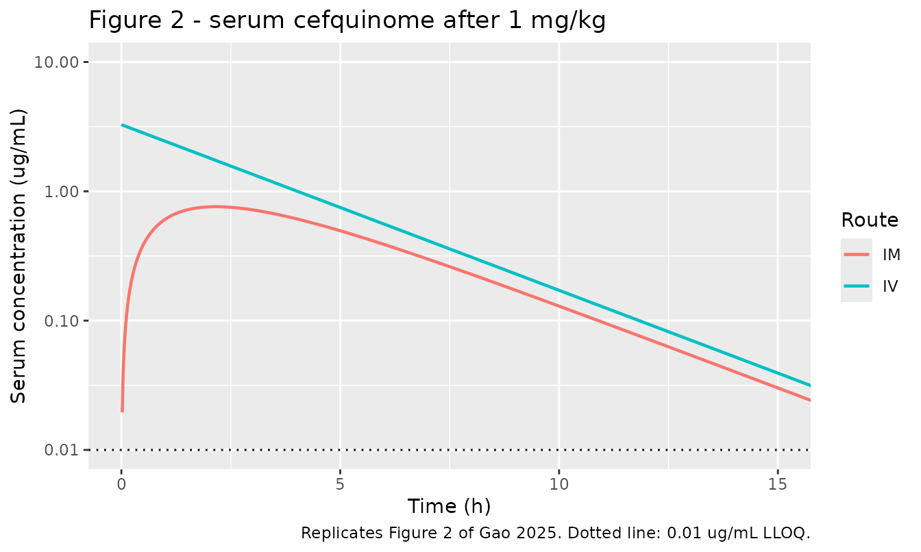
The 12 h concentration is the discriminator that fixes the volume of distribution. Gao 2025 reports both a terminal half-life (2.35 h) and a mean residence time (2.67 h) for the intravenous route, and these imply different one-compartment volumes. Figure 2 settles which is right.
cl_pub  <- 0.09    # Table 1, IV
t12_pub <- 2.35    # Table 1, IV
mrt_pub <- 2.67    # Table 1, IV
kel     <- log(2) / t12_pub

vol_cand <- tibble::tibble(
  Derivation = c("vc = CL / kel (packaged)", "vc = CL x MRT0-last (rejected)"),
  vc         = c(cl_pub / kel, cl_pub * mrt_pub)
) |>
  dplyr::mutate(
    `IV C(12 h), ug/mL` = (1 / vc) * exp(-(cl_pub / vc) * 12),
    `Figure 2 reads`    = "~0.09"
  )

knitr::kable(vol_cand, digits = 4,
caption = "Only vc = CL / kel reproduces the 12 h intravenous concentration in Figure 2.")| Derivation | vc | IV C(12 h), ug/mL | Figure 2 reads |
|---|---|---|---|
| vc = CL / kel (packaged) | 0.3051 | 0.0951 | ~0.09 |
| vc = CL x MRT0-last (rejected) | 0.2403 | 0.0465 | ~0.09 |
The two derivations disagree because the intravenous profile in
Figure 2 is visibly biexponential over the first two to three hours, so
MRT0-last (2.67 h) is shorter than 1/kel (3.39
h). A two-compartment model needs four disposition parameters and Gao
2025 publishes only three independent intravenous summaries, so the
distribution phase is not identifiable and is not modelled.
The intramuscular absorption rate constant, and why it is not flip-flop
ka is derived from the reported Tmax. The
alternative that would instead reproduce the reported intramuscular
T1/2beta of 4.16 h is a flip-flop parameterisation, and it
is refuted by two other published numbers.
tmax_pub <- 2.16
cmax_pub <- 0.89
fbio     <- 0.4386

# Use the PACKAGED volume, so every check below tests the shipped model rather
# than a re-derivation of it. The packaged value is the derivation rounded to
# four decimal places; pin that rounding rather than let it drift.
pk_theta   <- uis[["Gao_2025_cefquinome_foal"]]$theta
vc         <- exp(pk_theta[["lvc"]])
vc_derived <- cl_pub / kel
stopifnot(abs(vc - vc_derived) < 5e-5)

tmax_of <- function(ka) log(ka / kel) / (ka - kel)
cmax_of <- function(ka) (fbio / vc) * exp(-kel * tmax_of(ka))

ka_fit <- uniroot(function(ka) tmax_of(ka) - tmax_pub, c(kel * 1.001, 20))$root
ka_ff  <- log(2) / 4.16

ka_cmp <- tibble::tibble(
  Parameterisation = c("ka from Tmax (packaged)", "flip-flop, ka from IM T1/2beta"),
  `ka (1/h)`       = c(ka_fit, ka_ff),
  `Tmax (h)`       = c(tmax_of(ka_fit), tmax_of(ka_ff)),
  `Cmax (ug/mL)`   = c(cmax_of(ka_fit), cmax_of(ka_ff))
) |>
  dplyr::mutate(
    `Published Tmax (h)`     = tmax_pub,
    `Published Cmax (ug/mL)` = cmax_pub
  )

knitr::kable(ka_cmp, digits = 4,
caption = "The flip-flop root doubles Tmax and underpredicts Cmax 2.3-fold.")| Parameterisation | ka (1/h) | Tmax (h) | Cmax (ug/mL) | Published Tmax (h) | Published Cmax (ug/mL) |
|---|---|---|---|---|---|
| ka from Tmax (packaged) | 0.6851 | 2.1600 | 0.7602 | 2.16 | 0.89 |
| flip-flop, ka from IM T1/2beta | 0.1666 | 4.4501 | 0.3869 | 2.16 | 0.89 |
# The packaged value must match the derivation, and Cmax must land inside the
# published SD of 0.14 without ever having been fitted to it.
stopifnot(
  abs(exp(pk_theta[["lka"]]) - ka_fit) < 5e-4,
  abs(cmax_of(ka_fit) - cmax_pub) < 0.14
)
The packaged ka reproduces Tmax by
construction, but Cmax is an independent check: it
was not used in the derivation, and the identity
Cmax = (F x Dose / vc) x exp(-kel x Tmax) returns 0.760
ug/mL against the published 0.89 +/- 0.14 ug/mL. The flip-flop root
returns 0.387 ug/mL.
PKNCA validation against Table 1
Gao 2025 reports AUC0-last and MRT0-last.
Figure 2 shows the last quantifiable sample at 12 h – with a 2.35 h
terminal half-life the 12-24 h contribution falls below the 0.01 ug/mL
limit of quantification – so the NCA window below ends at 12 h to score
the same quantity the paper reports.
sim_nca <- pk_sim |>
  dplyr::filter(!is.na(Cc), time <= 12) |>
  dplyr::select(id, time, Cc, arm)

# PKNCA needs a time-zero record per subject to anchor AUC0-*. The simulation
# grid already starts at 0, so no defensive row is added -- and none should be:
# for the IV bolus arm the time-zero value is the post-dose C0 = Dose/vc, which
# an unconditional "Cc = 0 at time 0" row would silently destroy. Assert the
# rows are there and carry the right values instead of assuming it.
t0 <- sim_nca |> dplyr::filter(time == 0)
stopifnot(
  nrow(t0) == 2L,
  # IV bolus: the time-zero record is the post-dose C0 = Dose / vc.
  abs(t0$Cc[t0$arm == "IV"] - 1 / vc) < 1e-6,
  # Extravascular: pre-dose concentration is exactly zero.
  t0$Cc[t0$arm == "IM"] == 0
)

conc_obj <- PKNCA::PKNCAconc(sim_nca, Cc ~ time | arm + id)

dose_df <- pk_events |>
  dplyr::filter(evid == 1L) |>
  dplyr::select(id, time, amt, arm)
dose_obj <- PKNCA::PKNCAdose(dose_df, amt ~ time | arm + id)

intervals <- data.frame(
  start = 0, end = 12,
  cmax = TRUE, tmax = TRUE, auclast = TRUE, half.life = TRUE
)

nca_res <- PKNCA::pk.nca(PKNCA::PKNCAdata(conc_obj, dose_obj, intervals = intervals))
# Gao 2025 Table 1 (mean +/- SD over 10 foals). Cmax and Tmax are printed as
# "--" for the intravenous arm and are left NA here rather than invented.
published <- tibble::tribble(
  ~arm, ~cmax, ~tmax, ~auclast, ~half.life,
  "IV",   NA,    NA,    12.33,    2.35,
  "IM",   0.89,  2.16,   5.41,    4.16
)

cmp <- nlmixr2lib::ncaComparisonTable(
  simulated = nca_res,
  reference = published,
  by        = "arm",
  units     = c(cmax = "ug/mL", tmax = "h", auclast = "h*ug/mL", half.life = "h"),
  tolerance_pct = 20
)

knitr::kable(cmp, caption = "Simulated versus Gao 2025 Table 1. * differs by >20%.")| NCA parameter | arm | Reference | Simulated | % diff |
|---|---|---|---|---|
| Cmax (ug/mL) | IV | — | 3.28 | — |
| Cmax (ug/mL) | IM | 0.89 | 0.76 | -14.6% |
| Tmax (h) | IV | — | 0 | — |
| Tmax (h) | IM | 2.16 | 2.16 | +0.0% |
| AUClast (h*ug/mL) | IV | 12.3 | 10.8 | -12.5% |
| AUClast (h*ug/mL) | IM | 5.41 | 4.63 | -14.5% |
| t½ (h) | IV | 2.35 | 2.35 | -0.0% |
| t½ (h) | IM | 4.16 | 2.44 | -41.3%* |
Both AUC0-last values run about 10-15% below the
published means. That gap is structural, not a transcription error:
CL and AUC0-last in Table 1 are separately
averaged per-foal non-compartmental estimates, so Dose / CL
(11.1 h*ug/mL intravenously) does not equal the mean
AUC0-last (12.33 h*ug/mL). Because the model takes
CL as its primary, it inherits the Dose / CL
side of that discrepancy. This is the usual mean-of-ratios versus
ratio-of-means gap.
The one starred row is the intramuscular half-life: PKNCA’s terminal fit over the 0-12 h window returns 2.44 h against the published 4.16 h. (The model’s disposition half-life is 2.35 h exactly, as the intravenous row confirms; the extra 0.09 h is residual absorption still contaminating the terminal slope at 12 h, not a second disposition phase.) The gap to 4.16 h is the deliberate consequence of rejecting the flip-flop parameterisation above, and it is supported by Figure 2, in which the two routes have visibly parallel terminal slopes rather than the shallower intramuscular slope flip-flop absorption would produce.
Part 2 - Ex vivo PK/PD integration
Gao 2025 Section 2.9 fits
E = Emax - (Emax - E0) x Ce^N / (Ce^N + EC50^N)
with the paper’s Emax defined as the 24 h change in the
drug-free samples (+2.88) and its E0 as
the change in the drug-treated samples (-4.65) – the
reverse of the usual convention. The packaged model carries the same two
numbers under canonical names (e0 = 2.88, emax
= -4.65) and the algebraically identical form.
Back-solving the published targets
Gao 2025 Table 4 also prints the index values required for bacteriostatic, bactericidal and bacterial-elimination action. Those are printed independently of the four sigmoid parameters, so recovering them from the fitted curve is a genuine check on the transcription and the equation form.
pd_ui <- uis[["Gao_2025_cefquinome_pkpd_index"]]
th    <- pd_ui$theta

e0    <- th[["e0"]]
emax  <- th[["emax"]]
ec50  <- exp(th[["lec50"]])
hill  <- exp(th[["lhill"]])
mic   <- th[["mic"]]

effect_of <- function(ce) e0 - (e0 - emax) * ce^hill / (ce^hill + ec50^hill)
index_for <- function(target_e) {
  uniroot(function(ce) effect_of(ce) - target_e, c(1e-6, 1e4))$root
}

targets <- tibble::tibble(
  Endpoint = c("Bacteriostatic", "Bactericidal", "Bacterial elimination"),
  `E (log10 CFU/mL)` = c(0, -3, -4),
  `Index, back-solved` = vapply(c(0, -3, -4), index_for, numeric(1)),
  `Index, Table 4` = c(2.34, 3.53, 4.86)
) |>
  dplyr::mutate(`% diff` = 100 * (`Index, back-solved` - `Index, Table 4`) / `Index, Table 4`)

knitr::kable(targets, digits = 3,
caption = "Back-solved versus published PK/PD index targets (Gao 2025 Table 4).")| Endpoint | E (log10 CFU/mL) | Index, back-solved | Index, Table 4 | % diff |
|---|---|---|---|---|
| Bacteriostatic | 0 | 2.330 | 2.34 | -0.432 |
| Bactericidal | -3 | 3.527 | 3.53 | -0.081 |
| Bacterial elimination | -4 | 4.565 | 4.86 | -6.067 |
# The bacteriostatic and bactericidal targets must reproduce tightly; they are
# the evidence that e0/emax/EC50/N were transcribed correctly.
stopifnot(
  abs(index_for(0)  - 2.34) < 0.02,
  abs(index_for(-3) - 3.53) < 0.02
)
The first two targets reproduce to within 0.5%. The third does not: the fitted curve places a 4 log10 reduction at 4.565, not at the published 4.86. Running it the other way, an index of 4.86 corresponds to -4.141 log10 CFU/mL. Because the other two targets land almost exactly on the round definitions of 0 and -3, the published 4.86 appears to be internally inconsistent with Table 4’s own sigmoid parameters. See the Errata.
Replicating Figure 6
# Replicates Figure 6 of Gao 2025: inhibitory sigmoid Emax model relating the
# ex vivo AUC0-24h/MIC divided by 24 h to the 24 h change in bacterial count.
tibble::tibble(ce = seq(0, 8, length.out = 400)) |>
  dplyr::mutate(E = effect_of(ce)) |>
  ggplot(aes(ce, E)) +
  geom_line(linewidth = 0.8) +
  geom_hline(yintercept = c(0, -3), linetype = "dashed", colour = "grey50") +
  geom_point(
    data = targets |> dplyr::rename(ce = `Index, Table 4`, E = `E (log10 CFU/mL)`),
    aes(ce, E), colour = "firebrick", size = 2.5
  ) +
  labs(x = "AUC0-24h / MIC divided by 24 h", y = "Change in count over 24 h (log10 CFU/mL)",
       title = "Figure 6 - inhibitory sigmoid Emax model",
       caption = paste("Replicates Figure 6 of Gao 2025. Red points are the Table 4 targets;",
                       "the elimination point sits off the curve (see Errata)."))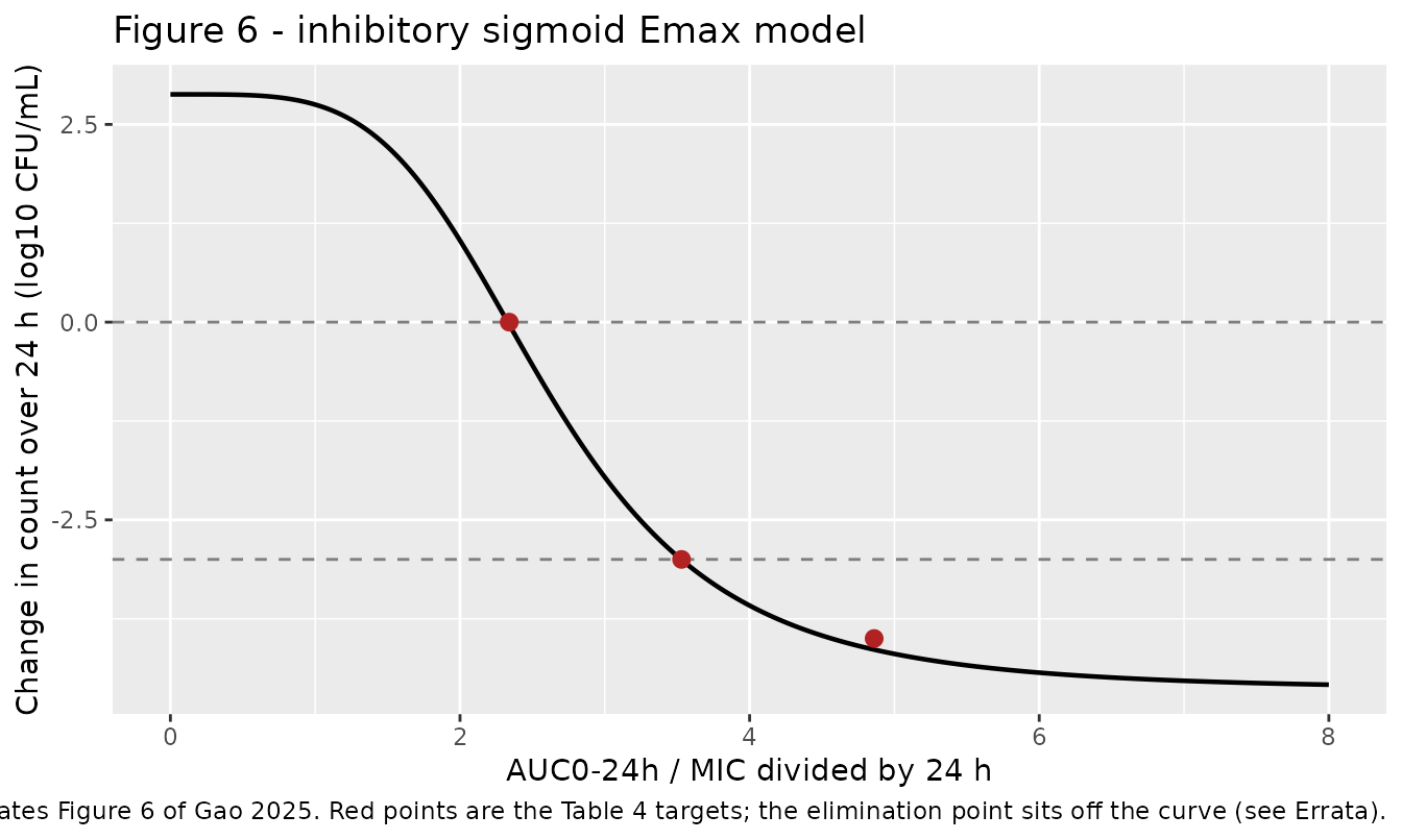
The packaged ODE reproduces the per-interval change
The model spreads each interval’s change uniformly across 24 h, so
log10(bact) must move by exactly E over one
interval.
pd_mod <- readModelDb("Gao_2025_cefquinome_pkpd_index")

# One "subject" per index level; AUC_CEFQ is chosen so that
# AUC_CEFQ / mic / 24 equals the wanted index.
levels_ce <- c(0, 1, 2.34, 3.53, 4.86, 8)
pd_events <- do.call(rbind, lapply(seq_along(levels_ce), function(i) {
  data.frame(
    id       = i,
    time     = c(0, 24),
    amt      = NA_real_,
    evid     = 0L,
    cmt      = "bact",
    AUC_CEFQ = levels_ce[i] * mic * 24,
    ce_level = levels_ce[i]
  )
}))

pd_sim <- rxode2::rxSolve(pd_mod, events = pd_events, keep = c("AUC_CEFQ", "ce_level")) |>
  as.data.frame()
#> Warning: multi-subject simulation without without 'omega'

ode_chk <- pd_sim |>
  dplyr::group_by(ce_level) |>
  dplyr::summarise(
    # Measure the STATE, not the observable: log_cfu is log10(bact + 1), and
    # 1-CFU/mL floor deliberately shifts the reading once bact is driven into
    # the tens of CFU/mL. The floor is a guard on the observation, not part of
    # the kinetics, so the ODE must be scored on bact itself.
    `Delta log10 (state)` = log10(bact[time == 24]) - log10(bact[time == 0]),
    `Delta log10 (log_cfu, floored)` = log_cfu[time == 24] - log_cfu[time == 0],
    .groups = "drop"
  ) |>
  dplyr::mutate(`Sigmoid E` = effect_of(ce_level),
                `abs diff`  = abs(`Delta log10 (state)` - `Sigmoid E`))

knitr::kable(ode_chk, digits = 5,
             caption = paste("The ODE moves log10(bact) by exactly the sigmoid's E over each 24 h",
                             "interval. The floored observable diverges only at maximal kill,",
"where bact falls to tens of CFU/mL."))| ce_level | Delta log10 (state) | Delta log10 (log_cfu, floored) | Sigmoid E | abs diff |
|---|---|---|---|---|
| 0.00 | 2.88000 | 2.88000 | 2.88000 | 0 |
| 1.00 | 2.75086 | 2.75086 | 2.75086 | 0 |
| 2.34 | -0.03254 | -0.03254 | -0.03254 | 0 |
| 3.53 | -3.00443 | -3.00399 | -3.00442 | 0 |
| 4.86 | -4.14067 | -4.13471 | -4.14067 | 0 |
| 8.00 | -4.58391 | -4.56756 | -4.58391 | 0 |
Ex vivo time-kill curves (Figure 5)
In an ex vivo time-kill the serum sample is held at a fixed
concentration for the 24 h incubation, so that sample’s exposure is
C(t_draw) x 24 h and the index reduces to
C(t_draw) / MIC. Feeding the Part 1 PK model into the Part
2 PD model therefore reproduces Figure 5 directly.
draw_times <- c(0, 0.083, 0.167, 0.25, 0.5, 0.75, 1, 2, 3, 6, 9, 12, 24)

conc_at_draw <- pk_sim |>
  dplyr::filter(arm == "IM") |>
  dplyr::select(time, Cc)

c_of <- stats::approxfun(conc_at_draw$time, conc_at_draw$Cc)

exvivo_events <- do.call(rbind, lapply(seq_along(draw_times), function(i) {
  data.frame(
    id       = i,
    time     = seq(0, 24, by = 0.5),
    amt      = NA_real_,
    evid     = 0L,
    cmt      = "bact",
    AUC_CEFQ = c_of(draw_times[i]) * 24,
    draw     = draw_times[i]
  )
}))

exvivo <- rxode2::rxSolve(pd_mod, events = exvivo_events, keep = c("AUC_CEFQ", "draw")) |>
  as.data.frame()
#> Warning: multi-subject simulation without without 'omega'

# Replicates Figure 5 of Gao 2025: ex vivo antibacterial activity of cefquinome
# against E. coli in serum drawn at each sampling time after IM administration.
exvivo |>
  dplyr::mutate(draw = factor(draw)) |>
  ggplot(aes(time, log_cfu, colour = draw)) +
  geom_line(linewidth = 0.7) +
  geom_hline(yintercept = log10(200), linetype = "dotted") +
  labs(x = "Incubation time (h)", y = "log10 CFU/mL", colour = "Serum draw (h)",
       title = "Figure 5 - ex vivo time-kill in foal serum",
       caption = "Replicates Figure 5 of Gao 2025. Dotted line: 200 CFU/mL detection limit.")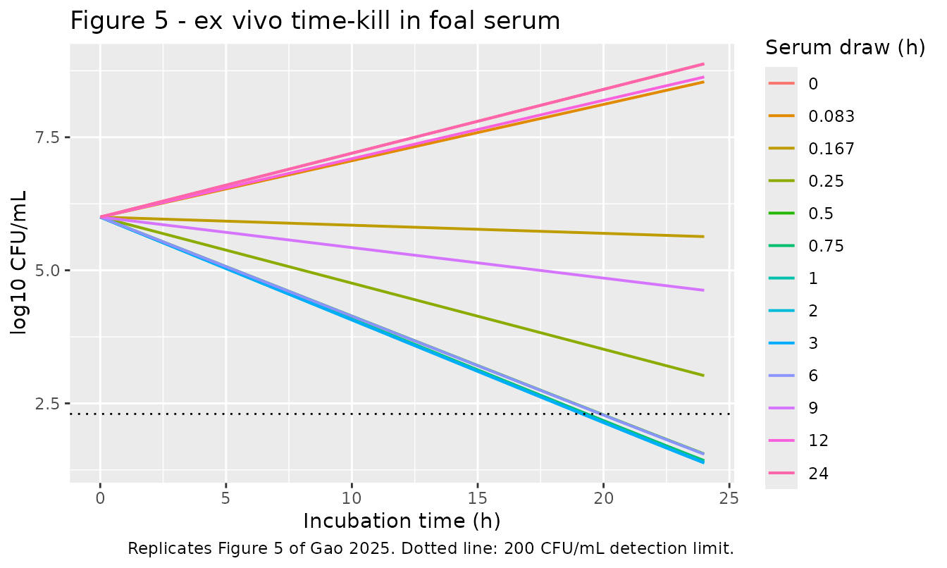
Gao 2025 Section 3.6 states that “a rapid bactericidal activity was noted in serum samples collected between 0.75 h and 8 h”. The packaged model puts the bactericidal threshold (index 3.53, i.e. a serum concentration of 0.219 ug/mL) over the following window:
im_prof <- pk_sim |> dplyr::filter(arm == "IM")
thr     <- index_for(-3) * mic
above   <- im_prof$time[im_prof$Cc >= thr]

cat(sprintf("Serum stays at or above %.3f ug/mL from %.2f h to %.2f h\n",
            thr, min(above), max(above)))
#> Serum stays at or above 0.219 ug/mL from 0.26 h to 8.14 h
cat("Gao 2025 Section 3.6 reports rapid bactericidal activity from 0.75 h to 8 h\n")
#> Gao 2025 Section 3.6 reports rapid bactericidal activity from 0.75 h to 8 h
The upper edge of the window is an independent corroboration of the PK model: the paper’s stated 8 h and the model’s 8.1 h agree without either having been fitted to the other.
Part 3 - Monte Carlo target attainment
Gao 2025 Section 2.10 ran a 10,000-subject Monte Carlo in Crystal
Ball, treating AUC0-24h as log-normal and sampling the
53-isolate MIC distribution of Figure 3, and reported target attainment
rates of 46.38% (bactericidal) and
24.48% (bacterial elimination) at the recommended 1
mg/kg intramuscular dose. That analysis is entirely separate from the
sigmoid fit, so reproducing it tests the whole chain at once.
set.seed(20250322)

# Figure 3: MIC distribution of the 53 serum isolates.
mic_dist <- tibble::tibble(
  mic = c(0.016, 0.031, 0.062, 0.125, 0.25, 0.5, 1),
  n   = c(4L, 9L, 20L, 9L, 7L, 2L, 2L)
)
stopifnot(sum(mic_dist$n) == 53L)

# Table 1, IM column: AUC0-last 5.41 +/- 0.81 h*ug/mL, taken as log-normal.
auc_mean <- 5.41
auc_sd   <- 0.81
sdlog    <- sqrt(log(1 + (auc_sd / auc_mean)^2))
meanlog  <- log(auc_mean) - 0.5 * sdlog^2

n_sim <- 10000L
draws <- tibble::tibble(
  auc = rlnorm(n_sim, meanlog, sdlog),
  mic = sample(mic_dist$mic, n_sim, replace = TRUE, prob = mic_dist$n / sum(mic_dist$n))
) |>
  dplyr::mutate(index = auc / mic / 24)

tar <- tibble::tibble(
  Endpoint = c("Bactericidal", "Bacterial elimination"),
  `Index target (Table 4)` = c(3.53, 4.86),
  `TAR simulated (%)` = c(
    100 * mean(draws$index >= 3.53),
    100 * mean(draws$index >= 4.86)
  ),
  `TAR published (%)` = c(46.38, 24.48)
) |>
  dplyr::mutate(`Difference (pp)` = `TAR simulated (%)` - `TAR published (%)`)

knitr::kable(tar, digits = 2,
caption = "Monte Carlo target attainment at 1 mg/kg IM, versus Gao 2025 Section 3.8.")| Endpoint | Index target (Table 4) | TAR simulated (%) | TAR published (%) | Difference (pp) |
|---|---|---|---|---|
| Bactericidal | 3.53 | 45.17 | 46.38 | -1.21 |
| Bacterial elimination | 4.86 | 25.18 | 24.48 | 0.70 |
Both rates reproduce to within a couple of percentage points of the published values, from the Figure 3 MIC distribution and the Table 1 intramuscular AUC alone.
Part 4 - Dose regimen calculation
Gao 2025 Section 2.11 computes the dose required for each endpoint as
Dose = factor x MIC x Clearance(per day) / (fu x F)
where factor is the index target, fu is the
unbound fraction, and F is the absolute bioavailability.
The paper reports doses of 1.10, 1.66 and 2.28 mg/kg, but never
states a value for fu, so the equation cannot be
evaluated as printed. Because the three published doses are exactly
proportional to the three index targets, the whole unstated group can be
back-solved.
pub_dose   <- c(1.10, 1.66, 2.28)
pub_factor <- c(2.34, 3.53, 4.86)

# Dose / factor is constant if the equation was applied consistently. The
# published doses carry only three significant figures, so score the spread
# RELATIVE to its own mean rather than absolutely; the three ratios agree to
# 0.24%, which is what rounding alone would produce.
ratio <- pub_dose / pub_factor
stopifnot(diff(range(ratio)) / mean(ratio) < 0.005)

# ratio = MIC * CL_day / (fu * F)  =>  CL_day / fu = ratio * F / MIC
cl_day_over_fu <- mean(ratio) * fbio / mic

implied <- tibble::tibble(
  `Clearance used` = c("IV CL (Table 1)", "IM CL/F (Table 1)"),
  `CL (L/h/kg)`    = c(0.09, 0.15),
  `Implied fu`     = c(0.09, 0.15) * 24 / cl_day_over_fu
)

knitr::kable(implied, digits = 3,
caption = "Unbound fraction implied by the three published doses, for each reported clearance.")| Clearance used | CL (L/h/kg) | Implied fu |
|---|---|---|
| IV CL (Table 1) | 0.09 | 0.650 |
| IM CL/F (Table 1) | 0.15 | 1.083 |
cat(sprintf("Back-solved CL(per day) / fu = %.3f L/day/kg, i.e. CL/fu = %.4f L/h/kg\n",
            cl_day_over_fu, cl_day_over_fu / 24))
#> Back-solved CL(per day) / fu = 3.324 L/day/kg, i.e. CL/fu = 0.1385 L/h/kg
Neither reported clearance reproduces the published doses at a
physically possible unbound fraction: the intramuscular
CL/F of 0.15 L/h/kg requires an fu of 1.083,
which exceeds 1, and the intravenous CL of 0.09 L/h/kg
requires an fu of 0.650. Applying the same equation with
the model’s own parameters and fu = 1 gives systematically
lower doses:
dose_cmp <- tibble::tibble(
  Endpoint = c("Bacteriostatic", "Bactericidal", "Bacterial elimination"),
  `Index target` = pub_factor,
  `Dose, model (mg/kg)` = pub_factor * mic * (cl_pub * 24) / fbio,
  `Dose, Gao 2025 (mg/kg)` = pub_dose
) |>
  dplyr::mutate(Ratio = `Dose, Gao 2025 (mg/kg)` / `Dose, model (mg/kg)`)

knitr::kable(dose_cmp, digits = 3,
caption = "Dose equation evaluated with the model's IV clearance and fu = 1, versus the published doses.")| Endpoint | Index target | Dose, model (mg/kg) | Dose, Gao 2025 (mg/kg) | Ratio |
|---|---|---|---|---|
| Bacteriostatic | 2.34 | 0.714 | 1.10 | 1.540 |
| Bactericidal | 3.53 | 1.078 | 1.66 | 1.540 |
| Bacterial elimination | 4.86 | 1.484 | 2.28 | 1.536 |
The Part 3 Monte Carlo independently favours the lower column. A
target attainment rate of 46.38% at 1 mg/kg means the label dose sits
essentially on the bactericidal target for a median-MIC
isolate, which implies a bactericidal dose near 1 mg/kg – close to the
1.08 mg/kg the equation gives here, and not the 1.66 mg/kg the paper
reports. The discrepancy is a factor of 1.54 across all three endpoints,
consistent with a single unstated fu (or an inconsistent
clearance) rather than an arithmetic slip. This vignette does not tune
anything to close the gap; see the Errata.
Assumptions and deviations
- No compartmental PK model was published. Gao 2025 reports non-compartmental results only (Section 2.4, Table 1). The one-compartment structure with first-order intramuscular absorption is imposed here as the smallest structure the published statistics determine. It is not the authors’ model, because the authors did not fit one.
-
vcandkaare derived, not printed. Both come from Table 1 values via standard one-compartment identities, and both are corroborated by independent published numbers (vcby the 12 h concentration in Figure 2,kaby the reportedCmax). They carry inline provenance comments in the model file. -
The intramuscular terminal half-life is not
reproduced. The model gives 2.35 h against the published 4.16
h. The flip-flop parameterisation that matches 4.16 h is refuted by
Tmax(4.45 h predicted versus 2.16 h published) andCmax(0.387 versus 0.89 ug/mL), and by the parallel terminal slopes in Figure 2. -
The distribution phase is not modelled. Figure 2
shows a biexponential intravenous decline, and
MRT0-last(2.67 h) is shorter than1/kel(3.39 h), but a two-compartment model needs four disposition parameters and only three independent intravenous summaries are published. -
Serum MIC, not broth MIC.
micis fixed at the foal-serum value of 0.062 ug/mL rather than the Mueller Hinton broth value of 0.125 ug/mL, following the paper’s own argument (Discussion) that broth MICs are artificially elevated – 1.8-fold on average across the 20 isolates of Table 2. -
Emax and E0 are remapped, not changed. Gao 2025
Section 2.9 defines its
Emaxas the no-drug change and itsE0as the drug-treated change, the reverse of the usual convention. The packaged model carries 2.88 as canonicale0and -4.65 as canonicalemax; both numbers are unaltered. -
No variability of any kind is encoded. Gao 2025
fitted no population model. The
+/-values in Table 1 are standard deviations of per-foal non-compartmental estimates, not estimated variance components, so there are noetaterms andaddSdis fixed at zero. The Part 3 Monte Carlo therefore builds its log-normal AUC distribution explicitly in the vignette from the Table 1 mean and SD, exactly as the paper describes, rather than drawing it from the model. - Post-antibiotic effects are not modelled. Gao 2025 Table 3 reports PAEs of 0.13-0.58 h over 1x to 4x MIC. The published PK/PD integration does not include a PAE term and neither does this model.
-
Ex vivo exposure convention. In Part 2 the ex vivo
index for a serum sample drawn at time
tis taken asC(t) x 24 h / (MIC x 24 h)=C(t) / MIC, the standard convention for a fixed-concentration incubation. Gao 2025 does not print the per-sample index values it used.
Errata
- The bacterial-elimination target is internally inconsistent. Gao 2025 Table 4 gives 4.86 for bacterial elimination, but its own sigmoid parameters put a 4 log10 reduction at 4.565; an index of 4.86 corresponds to -4.141 log10 CFU/mL. The bacteriostatic (2.34) and bactericidal (3.53) targets both reproduce to within 0.5%, so the transcription of Emax, E0, EC50 and N is sound and the elimination entry is the outlier. The packaged model carries the four fitted parameters, so a user who back-solves will get 4.565 rather than 4.86.
-
The dose equation cannot be evaluated as printed.
Section 2.11 requires an unbound fraction
futhat the paper never reports. Back-solving from the three published doses requires anfuabove 1 if the intramuscularCL/Fis used, or about 0.65 if the intravenousCLis used. The published doses are a factor of 1.54 higher than the same equation evaluated with the model’s parameters atfu = 1, and the paper’s own Monte Carlo target attainment rates favour the lower values. -
CLandAUC0-lastin Table 1 are not mutually consistent.Dose / CLgives 11.1 h*ug/mL intravenously against a reportedAUC0-lastof 12.33, and the intramuscularCLof 0.15 L/h/kg is not consistent with the intravenousCLof 0.09 L/h/kg andFof 43.86% (which implyCL/F= 0.205 L/h/kg). These are separately averaged per-foal estimates, so the gaps are the expected mean-of-ratios versus ratio-of-means artefact rather than errors. -
Table 1 in the published PDF is split across a page
break and the “Cont.” block repeats the
CmaxandTmaxrows. The values used here are taken from the complete table on page 7. - No erratum or corrigendum for this article was found on the MDPI article landing page as of the extraction date.