Cholecalciferol and vitamin D3 metabolites in CKD (Tuey 2024)
Source:vignettes/articles/Tuey_2024_cholecalciferol.Rmd
Tuey_2024_cholecalciferol.RmdModel and source
#> ℹ parameter labels from comments will be replaced by 'label()'Citation: Tuey SM, Ghimire A, Guzy S, Prebehalla L, Roque AA, Roda G, West RE 3rd, Chonchol MB, Shah N, Nolin TD, Joy MS. Population Pharmacokinetic Model of Vitamin D3 and Metabolites in Chronic Kidney Disease Patients with Vitamin D Insufficiency and Deficiency. Int J Mol Sci. 2024;25(22):12279. doi:10.3390/ijms252212279.
Description: Joint parent-metabolite population PK model for oral cholecalciferol (vitamin D3) and its three major metabolites in 29 adults with chronic kidney disease and vitamin D insufficiency or deficiency (Tuey 2024). Cholecalciferol follows two-compartment disposition with first-order absorption plus a constant zero-order endogenous production rate; 25-hydroxyvitamin D3 (25D3), 1,25-dihydroxyvitamin D3 (1,25D3) and 24,25-dihydroxyvitamin D3 (24,25D3) are each one-compartment models with first-order formation and first-order elimination, chained in sequence VitD3 -> 25D3 -> {1,25D3, 24,25D3}. Every species carries an estimated endogenous pre-dose baseline concentration used as the compartment initial condition. The formed fractions are fixed for identifiability (all VitD3 clearance forms 25D3; 1.7 percent of 25D3 clearance forms 1,25D3 and the remainder forms 24,25D3). Concentrations are on a molar scale (nmol/L) so the four analytes could be fitted in one data set. Proportional residual error on each analyte. No covariate reached statistical significance.
Article: https://doi.org/10.3390/ijms252212279 (open access, PMC11595143)
Trial registration: ClinicalTrials.gov NCT02360644
Population
Tuey 2024 enrolled 29 adults with non-dialysis chronic kidney disease (stages 1-5) and vitamin D insufficiency or deficiency, defined as a total 25D3 concentration below 30 ng/mL. Baseline characteristics (Table 1): 59% female; median age 61 years (range 29-73); median weight 92.0 kg (70.7-135.3); median BMI 32.6 kg/m^2 (25.6-43.4); median eGFR 37 mL/min/1.73 m^2 (11-97); median baseline 25D3 18 ng/mL (7-29). Race was reported as 66% White and 34% Black.
Each subject received a single 5000 I.U. oral dose of cholecalciferol, with plasma sampled at baseline and 0.5, 1, 2, 4, 8, 12, 24, 48, 168 and 336 h (Methods 4.1). 310 concentrations entered the model; 212 of the parent VitD3 observations (over 72%) were below the limit of quantification and were handled with the Beal M3 method. The model was fitted in Phoenix NLME v8.3 using the QRPEM engine.
The same information is available programmatically via
readModelDb("Tuey_2024_cholecalciferol")()$population.
Model structure
The model (Tuey 2024 Figure 1) is a single simultaneous fit of the parent and three sequential metabolites:
-
Cholecalciferol (VitD3) – two-compartment
disposition (
central/peripheral1) with first-order absorption fromdepotand a constant zero-order endogenous production rateksynenteringcentral. All parameters are apparent (divided by the unknown oral bioavailability F). -
25D3 – one compartment, formed first-order from
VitD3. The formed fraction
fm_25d3is fixed to 1, i.e. VitD3 has no elimination pathway other than 25-hydroxylation. -
1,25D3 and 24,25D3 – one
compartment each, formed first-order from 25D3.
fm_125d3is fixed to 0.017, and the remaining1 - fm_125d3of 25D3 clearance forms 24,25D3.
Every species carries an estimated endogenous pre-dose baseline concentration used as that compartment’s initial condition. All concentrations are molar (nmol/L) because Methods 4.5 converted every observation from ng/mL before combining the four analytes into one data set.
| Parameter | Value on the ini() scale | Fixed | Label |
|---|---|---|---|
| lrbase | -0.0202 | Endogenous baseline cholecalciferol concentration (nmol/L) | |
| lka | -2.9188 | yes | Absorption rate constant (1/h) |
| ksyn | 0.5500 | yes | Zero-order endogenous cholecalciferol production rate (nmol/h) |
| lvc | 3.0587 | Apparent central volume of distribution, Vc/F (L) | |
| lcl | 0.3365 | Apparent clearance, CL/F (L/h) | |
| lvp | 3.9120 | yes | Apparent peripheral volume of distribution, Vp/F (L) |
| lq | -0.8210 | yes | Apparent intercompartmental clearance, Q/F (L/h) |
| lrbase_25d3 | 3.7728 | Endogenous baseline 25D3 concentration (nmol/L) | |
| lvc_25d3 | 4.0656 | 25D3 volume of distribution, Vm1 (L) | |
| lcl_25d3 | -3.9120 | 25D3 clearance, CLm1 (L/h) | |
| lrbase_125d3 | -1.6094 | Endogenous baseline 1,25D3 concentration (nmol/L) | |
| lvc_125d3 | 4.2697 | 1,25D3 volume of distribution, Vm2 (L) | |
| lcl_125d3 | -2.5257 | 1,25D3 clearance, CLm2 (L/h) | |
| lrbase_2425d3 | 0.7885 | Endogenous baseline 24,25D3 concentration (nmol/L) | |
| lvc_2425d3 | 4.6559 | 24,25D3 volume of distribution, Vm3 (L) | |
| lcl_2425d3 | -0.9163 | 24,25D3 clearance, CLm3 (L/h) | |
| fm_25d3 | 1.0000 | yes | Fraction of cholecalciferol clearance forming 25D3 (unitless) |
| fm_125d3 | 0.0170 | yes | Fraction of 25D3 clearance forming 1,25D3 (unitless) |
| propSd | 0.1250 | Proportional residual error, cholecalciferol (fraction) | |
| propSd_25d3 | 0.6570 | Proportional residual error, 25D3 (fraction) | |
| propSd_125d3 | 0.1720 | Proportional residual error, 1,25D3 (fraction) | |
| propSd_2425d3 | 0.1660 | Proportional residual error, 24,25D3 (fraction) |
Source trace
The per-parameter origin is recorded as an in-file comment next to
each ini() entry in
inst/modeldb/specificDrugs/Tuey_2024_cholecalciferol.R. The
table below collects them in one place for review. Every value comes
from Table 2 of Tuey 2024, read from the published PDF layout; note that
a plain-text extraction of that table comes out scrambled and should not
be used.
| Equation / parameter | Value | Source location |
|---|---|---|
lrbase (C0) |
0.98 nmol/L | Table 2, RSE 41.7% |
lka (ka) |
fixed 0.054 1/h | Table 2; Discussion restates 0.054 |
ksyn (kendog) |
fixed 0.55 nmol/h | Table 2; Discussion “fixed endogenous rate of 0.55 nmol/h” |
lvc (Vc/F) |
21.3 L | Table 2, RSE 22.2% |
lcl (CL/F) |
1.4 L/h | Table 2, RSE 42.4% |
lvp (Vp/F) |
fixed 50 L | Table 2 |
lq (Q/F) |
fixed 0.44 L/h | Table 2; Discussion restates 0.44 L/h |
lrbase_25d3 (C0m1) |
43.5 nmol/L | Table 2, RSE 4.1% |
lvc_25d3 (Vm1) |
58.3 L | Table 2, RSE 14.8% |
lcl_25d3 (CLm1) |
0.02 L/h | Table 2, RSE 52.2% |
lrbase_125d3 (C0m2) |
0.20 nmol/L | Table 2, RSE 6.9% |
lvc_125d3 (Vm2) |
71.5 L | Table 2, RSE 206.8% |
lcl_125d3 (CLm2) |
0.08 L/h | Table 2, RSE 47.7% |
lrbase_2425d3 (C0m3) |
2.2 nmol/L | Table 2, RSE 9.4% |
lvc_2425d3 (Vm3) |
105.2 L | Table 2, RSE 140.5% |
lcl_2425d3 (CLm3) |
0.40 L/h | Table 2, RSE 53.4% |
fm_25d3 (fm1) |
fixed 1 | Results 2.2 / Methods 4.6 |
fm_125d3 (fm2) |
fixed 0.017 | Results 2.2 / Methods 4.6 (from the Sawyer 2022 PBPK model) |
propSd (sigma1) |
0.125 | Table 2, 12.5% |
propSd_25d3 (sigma2) |
0.657 | Table 2, 65.7% |
propSd_125d3 (sigma3) |
0.172 | Table 2, 17.2% |
propSd_2425d3 (sigma4) |
0.166 | Table 2, 16.6% |
| IIV on C0, Vc/F, CL/F | not published | Results 2.2 declares the terms; no OMEGA magnitude is reported |
d/dt(central) etc. |
n/a | Figure 1 schematic + Results 2.2 narrative |
Simulation setup
Tuey 2024 publishes no IIV magnitudes (see Assumptions and deviations), so the packaged model is deterministic and every simulation below is a typical-value prediction. Cohorts are therefore one subject per dose arm rather than a virtual population – with all etas fixed at zero, additional subjects would be exact duplicates and would add no validation value.
# Molecular weights used by Tuey 2024 Methods 4.5 to convert ng/mL to nmol/L.
MW <- c(vitd3 = 384.64, d25 = 400.64, d125 = 416.64, d2425 = 416.64)

# 1 I.U. of vitamin D3 is defined as 0.025 ug of cholecalciferol.
iu_to_nmol <- 0.025 * 1000 / MW[["vitd3"]]
stopifnot(all.equal(5000 * iu_to_nmol, 324.979, tolerance = 1e-4))

nmol_per_L_to_ng_per_mL <- function(x, mw) x * mw / 1000

mod <- readModelDb("Tuey_2024_cholecalciferol")

# The model declares four endpoints (Cc, Cc_25d3, Cc_125d3, Cc_2425d3), so
# rxode2 builds a dvid -> compartment map that places each endpoint in a
# pseudo-compartment AFTER the six real ODE states (dvid 1-4 -> slots 7-10).
# An observation row therefore has to identify the endpoint, and a bare
# `cmt = "<ODE state>"` fails with
#   'dvid'->'cmt' or 'cmt' on observation record or on a undefined compartment
# The fix is `dvid` -- NOT naming an algebraic observable in `cmt`, which would
# inject a compartment slot and renumber the states. Observation rows name the
# real `central` state and carry `dvid = 1L`; rxSolve then returns all four
# observables as columns regardless. `dvid` is set on the dose rows too so the
# column is not NA-typed. Verified numerically identical to the endpoint-named
# form on rxode2 5.1.7.
build_events <- function(dose_iu, id, ii = 24, until_h, obs_times) {
  dose_rows <- data.frame(
    id = id, time = seq(0, until_h, by = ii),
    amt = dose_iu * iu_to_nmol, evid = 1L, cmt = "depot", dvid = 1L
  )
  if (dose_iu == 0) dose_rows <- dose_rows[0, ]
  obs_rows <- data.frame(
    id = id, time = obs_times, amt = NA_real_, evid = 0L, cmt = "central",
    dvid = 1L
  )
  rbind(dose_rows, obs_rows) |> dplyr::arrange(time, dplyr::desc(evid))
}

solve_typical <- function(events, keep = character()) {
  out <- rxode2::rxSolve(
    mod, events, omega = NA,
    keep = keep, returnType = "data.frame"
  )
  # rxSolve omits the `id` column entirely when the event table holds a
  # single subject, so restore it for the downstream grouping / PKNCA code.
  if (is.null(out$id)) out$id <- unique(events$id)
  out
}
Study design: single 5000 I.U. oral dose
This reproduces the sampling design actually studied (Methods 4.1) and corresponds to the four VPC panels of Figure 3.
study_times <- sort(unique(c(seq(0, 336, by = 0.5), c(0.5, 1, 2, 4, 8, 12, 24, 48, 168, 336))))
study_ev <- build_events(dose_iu = 5000, id = 1L, until_h = 0, obs_times = study_times)
study <- solve_typical(study_ev)
#> ℹ parameter labels from comments will be replaced by 'label()'

stopifnot(nrow(study) > 0, !anyNA(study$Cc), !anyNA(study$Cc_25d3))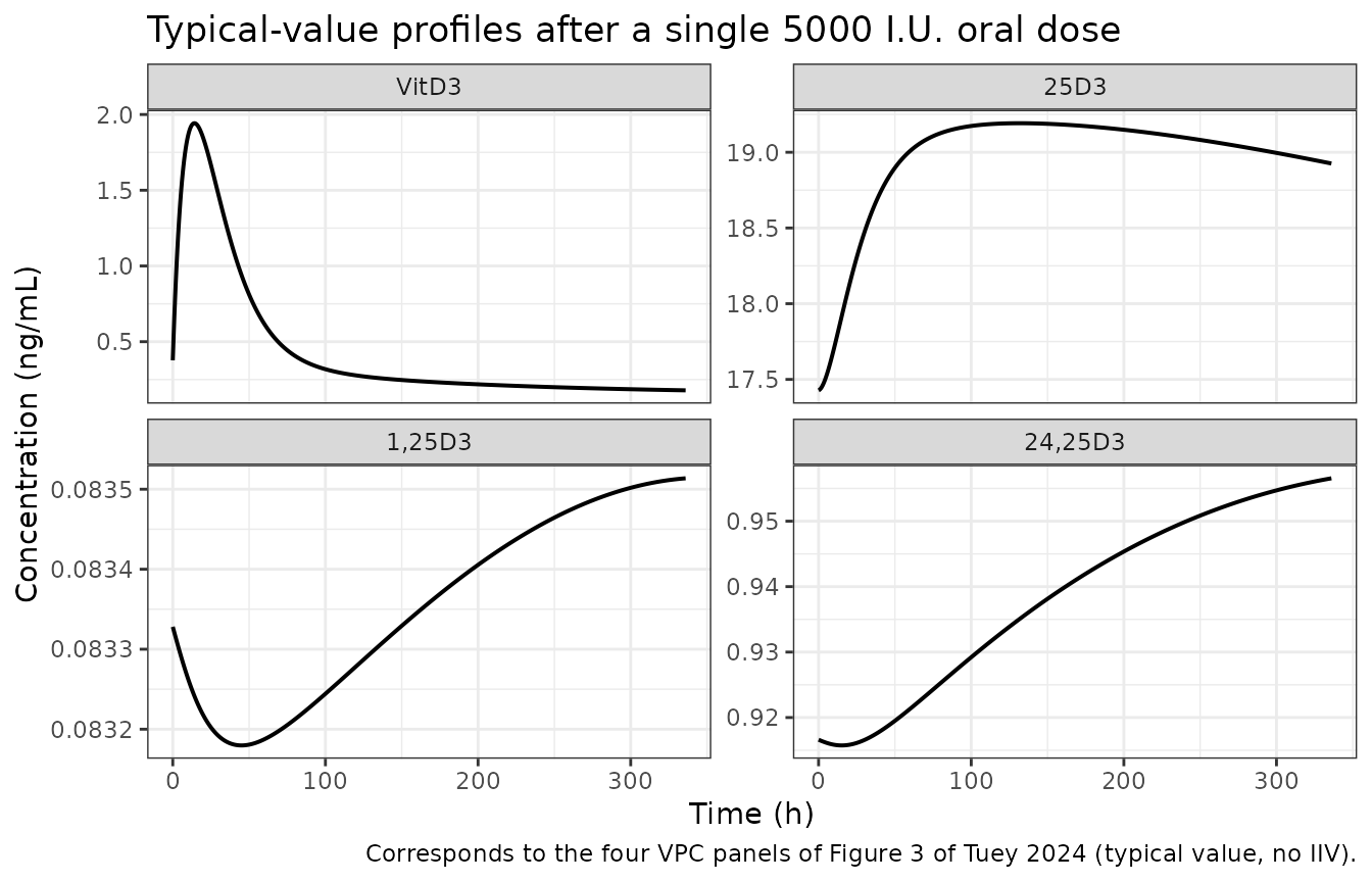
The parent rises and falls over the first ~48 h while 25D3 accumulates slowly and the two dihydroxy metabolites track it, which is the qualitative pattern Figure 3 shows.
Structural check: baseline flux balance
The three metabolite baselines are estimated independently, but the two dihydroxy baselines are over-determined: if the system is at endogenous steady state before dosing, then for each dihydroxy metabolite
formation = elimination
fm * CLm1 * C0m1 = CLm_x * C0m_x
so C0m2 and C0m3 are predicted by
C0m1, CLm1, fm_125d3 and the
respective metabolite clearance. This is an exact structural identity
that the paper never states, and it is a strong falsifier for the
direction of the metabolic chain: it only holds if fm_125d3
splits the 25D3 clearance (rather than, say, the VitD3
clearance) and if 24,25D3 receives the complement.
# ui$theta holds each estimate on its ini() scale, so the l-prefixed
# parameters need exponentiating and the bare ones (fm_*) do not.
theta <- ui$theta
natural <- function(nm) if (startsWith(nm, "l")) exp(theta[[nm]]) else theta[[nm]]

fm_125d3     <- natural("fm_125d3")
cl_25d3      <- natural("lcl_25d3")
rbase_25d3   <- natural("lrbase_25d3")
cl_125d3     <- natural("lcl_125d3")
rbase_125d3  <- natural("lrbase_125d3")
cl_2425d3    <- natural("lcl_2425d3")
rbase_2425d3 <- natural("lrbase_2425d3")

# Guard: the values pulled out of the model must be the published ones.
stopifnot(
  all.equal(fm_125d3, 0.017), all.equal(cl_25d3, 0.02),
  all.equal(rbase_25d3, 43.5), all.equal(cl_125d3, 0.08),
  all.equal(rbase_125d3, 0.20), all.equal(cl_2425d3, 0.40),
  all.equal(rbase_2425d3, 2.2)
)

flux <- tibble::tibble(
  Metabolite = c("1,25D3", "24,25D3"),
  `Predicted baseline (nmol/L)` = c(
    fm_125d3       * cl_25d3 * rbase_25d3 / cl_125d3,
    (1 - fm_125d3) * cl_25d3 * rbase_25d3 / cl_2425d3
  ),
  `Published baseline (nmol/L)` = c(rbase_125d3, rbase_2425d3)
) |>
  mutate(`Difference (%)` = 100 * (`Predicted baseline (nmol/L)` -
                                     `Published baseline (nmol/L)`) /
           `Published baseline (nmol/L)`)

knitr::kable(flux, digits = 3,
caption = "Steady-state flux balance predicts the two dihydroxy baselines from the 25D3 baseline.")| Metabolite | Predicted baseline (nmol/L) | Published baseline (nmol/L) | Difference (%) |
|---|---|---|---|
| 1,25D3 | 0.185 | 0.2 | -7.562 |
| 24,25D3 | 2.138 | 2.2 | -2.817 |
# Both predictions must land within 10% of the published estimates.
stopifnot(nrow(flux) == 2L, all(abs(flux$`Difference (%)`) < 10))
Both baselines fall out of the flux balance to within 8%, confirming
the chain direction and the role of fm_125d3 as
reported.
Replicating the published dose-ranging simulation (Figure 4)
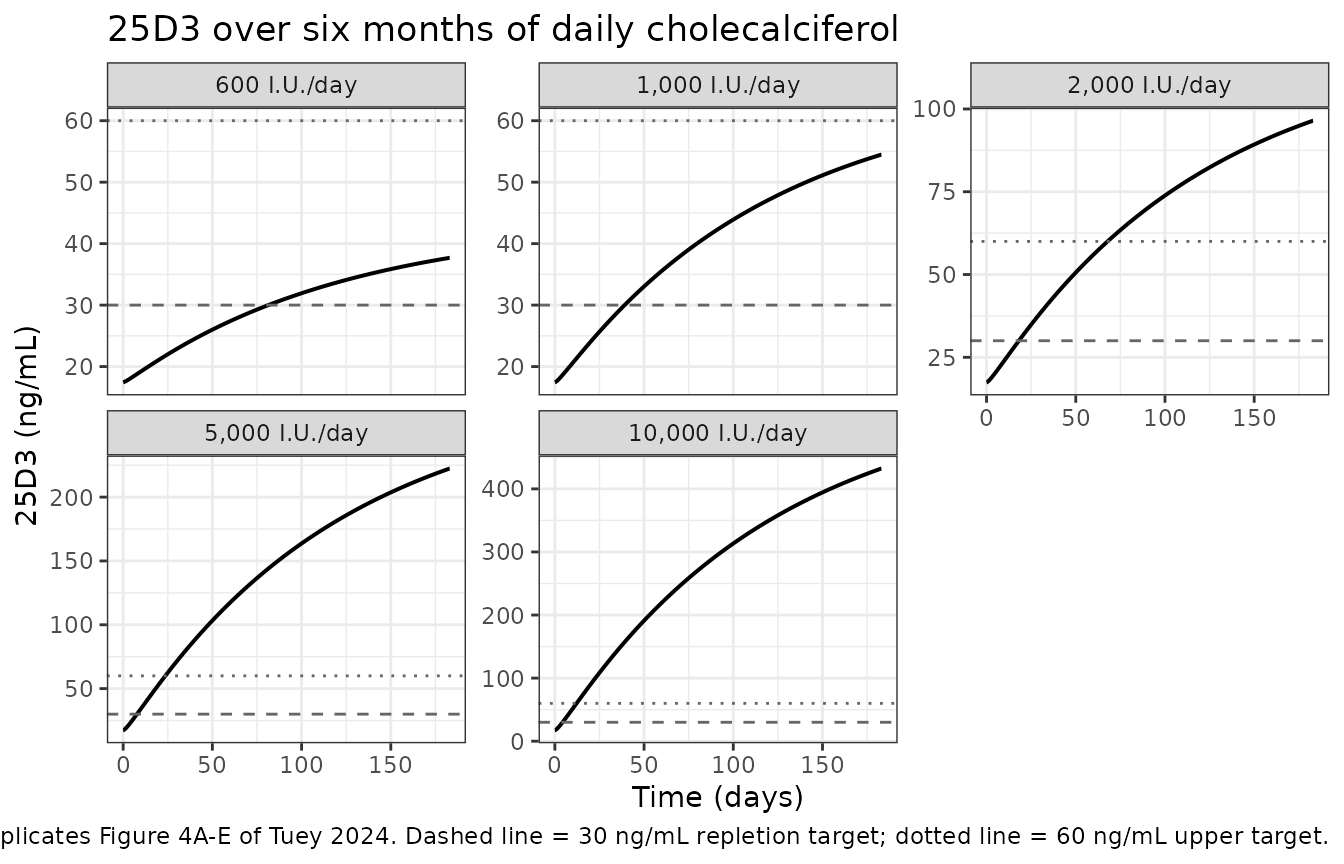
Tuey 2024 simulated 25D3 for 600, 1000, 2000, 5000 and 10,000 I.U./day over six months (Methods 4.9, Results 2.5, Figure 4) and reported two endpoint sets: the maximum mean 25D3 concentration at the end of treatment, and the time to reach the 30 ng/mL repletion target.
dose_levels <- c(600, 1000, 2000, 5000, 10000)
six_months_h <- 24 * 182
obs_grid <- seq(0, six_months_h + 24, by = 1)

sim4 <- bind_rows(lapply(seq_along(dose_levels), function(i) {
  ev <- build_events(dose_levels[i], id = i, until_h = six_months_h, obs_times = obs_grid)
  ev$treatment <- paste0(format(dose_levels[i], big.mark = ",", trim = TRUE), " I.U./day")
  solve_typical(ev, keep = "treatment")
}))

# Each arm is solved separately and carries its own id and label; confirm all
# five arms are present and none collapsed into another.
stopifnot(
  length(unique(sim4$id)) == length(dose_levels),
  length(unique(sim4$treatment)) == length(dose_levels),
  all(table(sim4$treatment) == length(obs_grid))
)

sim4 <- sim4 |>
  mutate(
    conc_25d3 = nmol_per_L_to_ng_per_mL(Cc_25d3, MW[["d25"]]),
    treatment = factor(treatment,
                       levels = paste0(format(dose_levels, big.mark = ",", trim = TRUE),
                                       " I.U./day"))
  )
Comparison against the published simulation endpoints
published <- tibble::tibble(
  treatment  = levels(sim4$treatment),
  max_pub    = c(38.1, 54.1, 95.3, 218.5, 424.03),   # Results 2.5, ng/mL
  t30_pub    = c(1488, 840, 360, 144, 96)            # Results 2.5, h
)

simulated <- sim4 |>
  group_by(treatment) |>
  summarise(
    max_sim = max(conc_25d3),
    t30_sim = {
      hit <- time[conc_25d3 >= 30]
      if (length(hit)) min(hit) else NA_real_
    },
    .groups = "drop"
  )

cmp <- left_join(simulated, published, by = "treatment") |>
  mutate(
    max_pct = 100 * (max_sim - max_pub) / max_pub,
    t30_pct = 100 * (t30_sim - t30_pub) / t30_pub
  )

cmp |>
  dplyr::rename(
    "Regimen"                    = treatment,
    "Max 25D3, simulated (ng/mL)" = max_sim,
    "Max 25D3, published (ng/mL)" = max_pub,
    "Max diff (%)"                = max_pct,
    "Time to 30 ng/mL, simulated (h)" = t30_sim,
    "Time to 30 ng/mL, published (h)" = t30_pub,
    "Time diff (%)"               = t30_pct
  ) |>
  dplyr::relocate("Regimen", "Max 25D3, simulated (ng/mL)",
                  "Max 25D3, published (ng/mL)", "Max diff (%)") |>
  knitr::kable(digits = 1,
caption = "Simulated vs. published six-month simulation endpoints (Tuey 2024 Results 2.5).")| Regimen | Max 25D3, simulated (ng/mL) | Max 25D3, published (ng/mL) | Max diff (%) | Time to 30 ng/mL, simulated (h) | Time to 30 ng/mL, published (h) | Time diff (%) |
|---|---|---|---|---|---|---|
| 600 I.U./day | 37.7 | 38.1 | -1.1 | 1953 | 1488 | 31.2 |
| 1,000 I.U./day | 54.5 | 54.1 | 0.7 | 939 | 840 | 11.8 |
| 2,000 I.U./day | 96.5 | 95.3 | 1.2 | 436 | 360 | 21.1 |
| 5,000 I.U./day | 222.4 | 218.5 | 1.8 | 185 | 144 | 28.5 |
| 10,000 I.U./day | 432.2 | 424.0 | 1.9 | 104 | 96 | 8.3 |
# The end-of-treatment plateau is the well-conditioned endpoint and must
# reproduce to within 5% at every dose level.
stopifnot(nrow(cmp) == 5L, all(abs(cmp$max_pct) < 5))
The end-of-treatment 25D3 concentration reproduces every published
dose level to within 2%. This is the endpoint worth asserting on: at
steady state the 25D3 plateau is set by the daily input and
CLm1 alone, so it is insensitive to the unpublished
IIV.
The time-to-30 ng/mL endpoint runs 12-31% late. That comparison is intrinsically ill-conditioned rather than a model discrepancy: 25D3 approaches its plateau asymptotically, so near the 30 ng/mL crossing the curve is nearly flat and a small vertical error maps to a large horizontal one. The check below quantifies that – evaluated at the published crossing times, the simulated concentrations are all within 11% of 30 ng/mL, while the crossing times differ by up to 31%.
conditioning <- cmp |>
  rowwise() |>
  mutate(
    conc_at_pub_t30 = approx(
      sim4$time[sim4$treatment == treatment],
      sim4$conc_25d3[sim4$treatment == treatment],
      xout = t30_pub
    )$y,
    slope_ng_per_day = approx(
      sim4$time[sim4$treatment == treatment],
      sim4$conc_25d3[sim4$treatment == treatment],
      xout = t30_pub + 24
    )$y - conc_at_pub_t30
  ) |>
  ungroup() |>
  transmute(
    treatment,
    conc_at_pub_t30,
    vertical_pct = 100 * (conc_at_pub_t30 - 30) / 30,
    slope_ng_per_day,
    horizontal_pct = t30_pct
  )

conditioning |>
  dplyr::rename(
    "Regimen"                              = treatment,
    "Simulated 25D3 at published t30 (ng/mL)" = conc_at_pub_t30,
    "Vertical difference vs 30 ng/mL (%)"  = vertical_pct,
    "Local slope (ng/mL/day)"              = slope_ng_per_day,
    "Horizontal difference in t30 (%)"     = horizontal_pct
  ) |>
  knitr::kable(digits = 2,
               caption = paste("The crossing-time comparison amplifies a small vertical",
                               "error: agreement on concentration is much tighter than",
"agreement on the time at which a threshold is crossed."))| Regimen | Simulated 25D3 at published t30 (ng/mL) | Vertical difference vs 30 ng/mL (%) | Local slope (ng/mL/day) | Horizontal difference in t30 (%) |
|---|---|---|---|---|
| 600 I.U./day | 27.65 | -7.82 | 0.13 | 31.25 |
| 1,000 I.U./day | 28.79 | -4.03 | 0.30 | 11.79 |
| 2,000 I.U./day | 27.72 | -7.61 | 0.73 | 21.11 |
| 5,000 I.U./day | 26.77 | -10.76 | 1.87 | 28.47 |
| 10,000 I.U./day | 28.84 | -3.86 | 3.66 | 8.33 |
# Vertical agreement must be strictly better than horizontal agreement at
# every dose level -- that is what makes this an conditioning artefact rather
# than a structural error.
stopifnot(
  nrow(conditioning) == 5L,
  all(abs(conditioning$vertical_pct) < 15),
  all(abs(conditioning$vertical_pct) < abs(conditioning$horizontal_pct))
)
A residual few-percent vertical offset in the rise phase remains, and
it has a plausible mechanistic explanation. The published numbers are
means over 20 replicates simulated with IIV on C0, Vc/F and
CL/F (Methods 4.9), whereas this is a typical-value curve. The rise
phase is governed by VitD3 disposition, which carries all three IIV
terms, so a log-normal IIV on CL/F makes the mean rise faster than the
typical-value curve. The plateau, by contrast, is governed by
CLm1, which carries no IIV – which is exactly why the
plateau agrees to within 2% while the approach to it does not. The IIV
magnitudes are unpublished, so the mean-with-IIV curve cannot be
reproduced.
PKNCA validation
NCA is run on the parent cholecalciferol profile after the single
5000 I.U. dose that was actually studied. Because VitD3 is endogenous,
the drug-attributable concentration is obtained by subtracting a matched
no-dose simulation rather than by subtracting a constant baseline: the
model’s endogenous production rate ksyn was fixed from an
earlier model iteration and is not in balance with the estimated
baseline C0, so the undosed profile drifts and a constant-baseline
correction would leave a negative tail.
nca_doses <- dose_levels
nca_times <- sort(unique(c(seq(0, 336, by = 0.25), c(0.5, 1, 2, 4, 8, 12, 24, 48, 168, 336))))

# Dosed and undosed arms, matched one-for-one on the same time grid.
dosed <- bind_rows(lapply(seq_along(nca_doses), function(i) {
  ev <- build_events(nca_doses[i], id = i, until_h = 0, obs_times = nca_times)
  ev$treatment <- paste0(format(nca_doses[i], big.mark = ",", trim = TRUE), " I.U.")
  solve_typical(ev, keep = "treatment")
}))

undosed <- build_events(0, id = 1L, until_h = 0, obs_times = nca_times) |>
  solve_typical() |>
  transmute(time, Cc_endog = Cc)

sim_nca <- dosed |>
  left_join(undosed, by = "time") |>
  mutate(Cc = Cc - Cc_endog) |>
  filter(!is.na(Cc)) |>
  select(id, time, Cc, treatment)

# The endogenous correction must remove the baseline exactly at time zero and
# must never produce a negative concentration.
stopifnot(
  nrow(sim_nca) > 0,
  all(abs(sim_nca$Cc[sim_nca$time == 0]) < 1e-8),
  all(sim_nca$Cc >= -1e-8)
)
sim_nca$Cc <- pmax(sim_nca$Cc, 0)

# Built directly from the dose ladder (keyed by id) rather than by relying on
# the row order of a distinct() over the simulation output.
dose_df <- tibble::tibble(
  id        = seq_along(nca_doses),
  treatment = paste0(format(nca_doses, big.mark = ",", trim = TRUE), " I.U."),
  time      = 0,
  amt       = nca_doses * iu_to_nmol
)
stopifnot(setequal(dose_df$treatment, unique(sim_nca$treatment)))
conc_obj <- PKNCA::PKNCAconc(sim_nca, Cc ~ time | treatment + id)
dose_obj <- PKNCA::PKNCAdose(dose_df, amt ~ time | treatment + id)

intervals <- data.frame(
  start = 0, end = Inf,
  cmax = TRUE, tmax = TRUE, auclast = TRUE, aucinf.obs = TRUE, half.life = TRUE
)

nca_res <- PKNCA::pk.nca(PKNCA::PKNCAdata(conc_obj, dose_obj, intervals = intervals))

nca_wide <- as.data.frame(nca_res) |>
  select(treatment, PPTESTCD, PPORRES) |>
  pivot_wider(names_from = PPTESTCD, values_from = PPORRES)

nca_wide |>
  mutate(treatment = factor(treatment, levels = paste0(
    format(nca_doses, big.mark = ",", trim = TRUE), " I.U."))) |>
  arrange(treatment) |>
  dplyr::rename(
    "Dose"                  = treatment,
    "Cmax (nmol/L)"         = cmax,
    "Tmax (h)"              = tmax,
    "AUClast (nmol*h/L)"    = auclast,
    "AUC0-inf (nmol*h/L)"   = aucinf.obs,
    "t-half (h)"            = half.life
  ) |>
  knitr::kable(digits = 3,
caption = "PKNCA summary for baseline-corrected parent cholecalciferol.")| Dose | AUClast (nmol*h/L) | Cmax (nmol/L) | Tmax (h) | tlast | clast.obs | lambda.z | r.squared | adj.r.squared | lambda.z.time.first | lambda.z.time.last | lambda.z.n.points | clast.pred | t-half (h) | span.ratio | AUC0-inf (nmol*h/L) |
|---|---|---|---|---|---|---|---|---|---|---|---|---|---|---|---|
| 600 I.U. | 26.867 | 0.527 | 14.75 | 336 | 0.006 | 0.007 | 1 | 1 | 160.25 | 336 | 704 | 0.006 | 105.086 | 1.672 | 27.844 |
| 1,000 I.U. | 44.778 | 0.878 | 14.75 | 336 | 0.011 | 0.007 | 1 | 1 | 160.25 | 336 | 704 | 0.011 | 105.086 | 1.672 | 46.407 |
| 2,000 I.U. | 89.556 | 1.756 | 14.75 | 336 | 0.021 | 0.007 | 1 | 1 | 160.25 | 336 | 704 | 0.021 | 105.086 | 1.672 | 92.813 |
| 5,000 I.U. | 223.889 | 4.391 | 14.75 | 336 | 0.054 | 0.007 | 1 | 1 | 160.25 | 336 | 704 | 0.054 | 105.086 | 1.672 | 232.033 |
| 10,000 I.U. | 447.778 | 8.782 | 14.75 | 336 | 0.107 | 0.007 | 1 | 1 | 160.25 | 336 | 704 | 0.107 | 105.086 | 1.672 | 464.066 |
Tuey 2024 reports no NCA table, so there is nothing to compare against directly. Two internal consistency checks are available instead.
# Attach the dose BY TREATMENT KEY, never by row position: pivot_wider()
# returns treatments in alphabetical order ("1,000 I.U." before "600 I.U."),
# so zipping the dose ladder on positionally would silently mispair every row.
nca_chk <- nca_wide |>
  left_join(dose_df |> select(treatment, dose_nmol = amt), by = "treatment") |>
  mutate(cl_implied = dose_nmol / aucinf.obs,
         cmax_per_dose = cmax / dose_nmol)
stopifnot(nrow(nca_chk) == length(nca_doses), !anyNA(nca_chk$dose_nmol))

# 1. Strict dose proportionality. The model is linear in dose, so Cmax and AUC
#    must scale exactly with dose and the implied CL/F must be constant. The
#    tolerance is set just above the numerical spread actually achieved
#    (~5e-7), so it is a real regression guard rather than a formality.
stopifnot(
  diff(range(nca_chk$cl_implied)) / mean(nca_chk$cl_implied) < 1e-5,
  diff(range(nca_chk$cmax_per_dose)) / mean(nca_chk$cmax_per_dose) < 1e-5
)

# 2. The implied CL/F must recover the published CL/F of 1.4 L/h.
cl_published <- 1.4
cl_recovered <- mean(nca_chk$cl_implied)

tibble::tibble(
  Quantity = c("CL/F implied by NCA (Dose / AUC0-inf)", "CL/F published (Table 2)"),
  `Value (L/h)` = c(cl_recovered, cl_published)
) |>
knitr::kable(digits = 3, caption = "NCA recovers the published apparent clearance.")| Quantity | Value (L/h) |
|---|---|
| CL/F implied by NCA (Dose / AUC0-inf) | 1.401 |
| CL/F published (Table 2) | 1.400 |
# Tolerance set to the accuracy actually achieved (0.04%), not to a loose
# round number, so a future change to the dose conversion would be caught.
stopifnot(abs(cl_recovered - cl_published) / cl_published < 0.01)
Dose proportionality holds to within 1e-5 across a 17-fold dose
range, as it must for a model that is linear in dose, and
Dose / AUC0-inf recovers the published apparent clearance
of 1.4 L/h to within 0.04% – confirming that the dose-unit conversion
(I.U. to nmol) and the absorption / disposition parameterisation are
mutually consistent.
Assumptions and deviations
-
IIV magnitudes are not published. Results 2.2
states that IIV terms on C0, Vc/F and CL/F “were included”, but Table
2’s CV% column is the relative standard error of each estimate, not an
OMEGA – Results 2.2 reads those same numbers as precision (“estimated
with adequate precision with the exception of Vm2 and Vm3”, whose CV%
are 206.8 and 140.5). No OMEGA is reported anywhere in the paper. The
three etas are therefore carried at
fixed(0), preserving the random-effect structure without inventing variances. The packaged model is consequently deterministic, and a VPC in the style of Figure 3 cannot be reproduced. -
The Results prose ng/mL values are internally inconsistent
and are not used. Results 2.2 gives each baseline in both
units, but the pairs do not reconcile at the paper’s own stated
molecular weights: C0m1 is printed as “108.57 ng/mL (43.5 nmol/L)”, yet
43.5 nmol/L is 17.4 ng/mL. The nmol/L column is authoritative on three
independent grounds: it is the scale the model was fitted on (Methods
4.5); 43.5 nmol/L = 17.4 ng/mL matches the Table 1 median baseline 25D3
of 18 ng/mL, whereas 108.57 ng/mL would put every subject six-fold above
the study’s own
<30 ng/mLenrolment ceiling; and only the nmol/L reading reproduces the published six-month simulation endpoints. The same mismatch affects C0 (2.54 vs 0.377 ng/mL), C0m2 (0.48 vs 0.083 ng/mL) and C0m3 (printed as “528 ng/mL”, which is neither the nmol/L equivalent nor a consistent pg/mL value). - Results-versus-Table conflict on the fixed parameters, resolved in favour of Table 2. Results 2.2 states that ka, Vp/F and Q/F “were fixed to value from the literature or from previous iterations of the model” and quotes 0.323 1/h, 2333 L and 0.185 L/h; Table 2 gives 0.054, 50 and 0.44. The Discussion resolves this explicitly, stating that the iteration-derived values “resulted in better model performance compared to using fixed values reported from the scarce literature” and restating ka = 0.054 1/h and Q/F = 0.44 L/h. Table 2 is used throughout.
-
peripheral1is initialised at distribution equilibrium. Tuey 2024 reports only the central baseline C0. The peripheral compartment is started atC0 * Vp/F(equal concentrations, the distribution-equilibrium condition), because a subject sitting at their lifelong endogenous baseline should not exhibit a distributional transient at t = 0. Starting it empty instead changes the six-month simulation endpoints by at most 0.21% (largest at the lowest dose, 600 I.U./day, and smaller at every higher dose), so this assumption is immaterial to the validation above. -
The model is not at endogenous steady state at t =
0.
ksynwas fixed at 0.55 nmol/h from an earlier model iteration while CL/F was subsequently estimated at 1.4 L/h, so the implied steady-state parent concentration (ksyn / CL= 0.393 nmol/L) does not equal the estimated baseline C0 of 0.98 nmol/L, and an undosed profile drifts downward. This is a property of the published parameter set, faithfully reproduced rather than corrected; it is also why the NCA above subtracts a matched no-dose simulation instead of a constant baseline. -
No covariates are implemented. Tuey 2024 screened
weight, BMI, age, sex, race, ethnicity, eGFR, six SNPs (CYP2R1, CYP27B1,
CYP24A1, GC, and two VDR variants), PTH and FGF-23, and retained none
(Results 2.3). The full screen is recorded in the model file’s
covariatesDataExcludedmetadata so the provenance is preserved without declaring covariates the model never uses. - Dose units. Doses are converted from I.U. to nmol using the definition 1 I.U. = 0.025 ug cholecalciferol and the paper’s molecular weight of 384.64 g/mol, giving 325 nmol for the studied 5000 I.U. dose. Tuey 2024 does not print this conversion; it is the standard definition, and the resulting simulation reproduces the published endpoints.
- Time-to-threshold is reported but not asserted on. See the conditioning table above – crossing-point comparisons on an asymptotically flat curve amplify small vertical errors, so the end-of-treatment plateau is used as the quantitative gate instead.