Lenvatinib dose finding in hepatocellular carcinoma (Tamai 2017)
Source:vignettes/articles/Tamai_2017_lenvatinib.Rmd
Tamai_2017_lenvatinib.RmdModels and source
Tamai 2017 is a two-part dose-finding analysis, and it contributes
two model files to nlmixr2lib:
-
Tamai_2017_lenvatinib– the population PK model, a three-compartment model with sequential zero-order release into a depot followed by first-order absorption, re-estimated on 8761 concentrations from 452 subjects. -
Tamai_2017_lenvatinib_teae_dosemod– the landmark logistic exposure-safety model for a cycle-1 treatment-emergent adverse event (TEAE) forcing lenvatinib withdrawal or dose reduction, fitted in the 45 evaluable subjects of the phase 2 part of study 202.
The paper chains them: the PK model produces each subject’s steady-state AUC, and that AUC is the sole predictor in the logistic model. A receiver operating characteristic (ROC) analysis then converts the two into a body-weight-banded starting-dose recommendation. This vignette reproduces that chain end to end.
- Citation: Tamai T, Hayato S, Hojo S, Suzuki T, Okusaka T, Ikeda K, Kumada H. Dose finding of lenvatinib in subjects with advanced hepatocellular carcinoma based on population pharmacokinetic and exposure-response analyses. J Clin Pharmacol. 2017;57(9):1138-1147. doi:10.1002/jcph.917.
- Article: https://doi.org/10.1002/jcph.917
- PubMed Central open access: https://www.ncbi.nlm.nih.gov/pmc/articles/PMC5575539/
pk_mod <- readModelDb("Tamai_2017_lenvatinib")
er_mod <- readModelDb("Tamai_2017_lenvatinib_teae_dosemod")
There are two sibling lenvatinib entries in the library.
Gupta_2016_lenvatinib is the predecessor
fit (reference 31 of this paper): the same structural model on 779
subjects from 15 studies, before study 202 existed. Tamai 2017 took that
model as its starting point and re-estimated it after adding the HCC
data, which is why the two parameter sets are close but not identical
and why the albumin term of the Gupta model is absent here.
Majid_2024_lenvatinib_* are downstream PK/PD models that
consume lenvatinib AUC as a driver.
Population
The PK analysis set pools 452 subjects and 8761 lenvatinib plasma concentrations from 13 studies (Tamai 2017 Table 1 and PK Data Set): 232 healthy adults contributing 5077 concentrations across 8 phase 1 clinical pharmacology studies, 155 subjects with mixed solid tumors contributing 3188 concentrations across 4 phase 1 dose-finding studies (NCT00121719, NCT00121680, NCT00280397, NCT01268293), and 65 subjects with advanced HCC Child-Pugh class A contributing 496 concentrations from study 202 (NCT00946153).
Baseline demographics (Table 1): age median 50.0 years (range 18.0 to 85.0), weight median 75.1 kg (range 42.7 to 147.0), 162 female and 290 male, race White 253 / Japanese 90 / Black 66 / Other 33 / Hispanic 6 / Other Asian 4. Alkaline phosphatase is strongly right-skewed – median 81.5 U/L against a mean of 160.4 – and creatinine clearance median is 103.6 mL/min. Concomitant CYP3A4 inducers were recorded in 16 of 452 subjects and CYP3A inhibitors in 34 of 452.
The exposure-response analysis set is much smaller: the 45 evaluable subjects of the phase 2 expansion of study 202, all dosed at lenvatinib 12 mg once daily in 4-week cycles, of whom 21 (46.7 percent) had a TEAE leading to dose reduction or discontinuation during cycle 1. Study 202 subjects had low body weight (median 58.8 kg) and 71 percent had alkaline phosphatase above the upper limit of normal.
The same information is available programmatically:
readModelDb("Tamai_2017_lenvatinib")()$population
readModelDb("Tamai_2017_lenvatinib_teae_dosemod")()$population
Source trace
Per-parameter origins are recorded as in-file comments beside each
ini() entry in
inst/modeldb/specificDrugs/Tamai_2017_lenvatinib.R and
inst/modeldb/specificDrugs/Tamai_2017_lenvatinib_teae_dosemod.R.
Collected here for review. Every population-PK value is the
Final Model column of Table 2, not the Base Model
column printed to its left, and each is cross-checked against the
bootstrap median in the rightmost column.
Population PK model (Tamai_2017_lenvatinib)
| Equation / parameter | Value | Source location |
|---|---|---|
lcl (CL/F) |
6.43 L/h | Table 2, final theta_CL (RSE 2.19%; bootstrap 6.42,
6.07-6.76) |
lvc (V1/F) |
47.0 L | Table 2, final theta_V1 (RSE 4.40%; bootstrap 46.8,
43.9-49.8) |
lvp (V2/F) |
31.2 L | Table 2, final theta_V2 (RSE 6.76%; bootstrap 31.1,
28.3-33.7) |
lvp2 (V3/F) |
34.5 L | Table 2, final theta_V3 (RSE 4.14%; bootstrap 34.7,
31.6-37.7) |
lq (Q1/F) |
3.96 L/h | Table 2, final theta_Q1 (RSE 3.03%; bootstrap 3.99,
3.57-4.49) |
lq2 (Q2/F) |
0.726 L/h | Table 2, final theta_Q2 (RSE 2.91%; bootstrap 0.738,
0.639-0.845) |
lka (Ka) |
1.04 1/h | Table 2, final Ka (RSE 6.80%; bootstrap 1.04,
0.933-1.13) |
ld1 (D1) |
1.06 h | Table 2, final D1 (RSE 5.77%; bootstrap 1.06,
0.987-1.14) |
lfdepot (F1) |
0.867 | Table 2, final F1, capsule vs tablet (RSE 1.00%;
bootstrap 0.867, 0.815-0.908) |
e_wt_cl |
0.708 | Table 2, final theta_WGT1, on CL/F, Q1/F, Q2/F (RSE
6.58%; bootstrap 0.711, 0.538-0.886) |
e_wt_vc_vp |
1.08 | Table 2, final theta_WGT2, on V1/F, V2/F, V3/F (RSE
5.42%; bootstrap 1.08, 0.876-1.28) |
e_cyp3a4_ind_cl |
log(1.30) | Table 2, final theta_INDU; Results: “+30% on CL/F” |
e_cyp3a4_inh_cl |
log(0.922) | Table 2, final theta_INHIB; Results: “-7.8% on
CL/F” |
e_dis_healthy_cl |
log(1.19) | Table 2, final theta_TM; Results: healthy subjects 19%
higher CL/F |
e_alp_cl |
log(0.852) | Table 2, final theta_ALP; Results: “-14.8% with ALP
above ULN” |
etalcl, etalvc block |
0.106276 / 0.096661 / 0.245025 | Table 2, final IIV 32.6% and 49.5% CV with footnote a; correlation R = 0.599 stated below the table |
etalvp |
0.389376 | Table 2, final IIV V2/F 62.4% CV |
etalvp2 |
0.176400 | Table 2, final IIV V3/F 42.0% CV |
etalka |
0.216225 | Table 2, final IIV Ka 46.5% CV |
etald1 |
0.467856 | Table 2, final IIV D1 68.4% CV |
propSd |
0.302 | Table 2, final proportional %CV, patient studies |
addSd |
7.35 ng/mL | Table 2, final additive term, time after dose <= 2 h |
| CL/F covariate equation | n/a | Table 2 row header:
CL/F = theta_CL * (WGT/75)^theta_WGT1 * theta_INDU^INDU * theta_INHIB^INHIB * theta_TM^TM * theta_ALP^ALP
|
| Three-compartment ODE, sequential zero- then first-order absorption | n/a | Methods, “PK Model for Lenvatinib” |
alp_uln = 120 U/L |
120 U/L |
NOT from Tamai 2017 – representative adult cutoff
carried from Gupta_2016_lenvatinib (see Assumptions and
deviations) |
Exposure-response model
(Tamai_2017_lenvatinib_teae_dosemod)
| Equation / parameter | Value | Source location |
|---|---|---|
logit_ref |
-4.71 | Results, “Exposure-Response Relationship Analysis …” final paragraph (RSE 29.3%; 95% CI -7.41 to -2.01) |
e_auc_len_logit |
1.82 per 1000 ng*h/mL
|
same paragraph (RSE 28.8%; 95% CI 0.793 to 2.85) |
logit = intercept + slope * AUC |
n/a | same paragraph, model form stated in words |
addSd_prob_teae_dosemod |
fixed(0.001) | NOT from Tamai 2017 – placeholder so rxode2 has an error model (see Assumptions and deviations) |
Structural interpretation of the IIV column deserves a note, because
two readings are in circulation. Table 2 footnote a states the
convention explicitly: “The %CV for both intersubject and proportional
residual variability is an approximation taken as the square root of the
variance x 100.” The omega variance is therefore the squared fraction
directly, (%CV/100)^2, and not the log-normal conversion
log(CV^2 + 1) that the sibling
Gupta_2016_lenvatinib applies. Check 2 below shows that the
paper’s own simulated AUC values are reproduced under this reading.
Virtual cohort
No individual data from study 202 are public. Two virtual cohorts are used.
The deterministic grid sweeps body weight from 40 to 120 kg – exactly the range Tamai 2017 states for its Figure 5 simulation – at both candidate starting doses, with all random effects zeroed. The stochastic cohort places 150 subjects at each of the four body-weight / dose corners the paper quotes numerically, so per-subject variability is carried through PKNCA.
Both use the HCC reference covariate setting: cancer patient
(DIS_HEALTHY = 0), no concomitant CYP3A modulator, alkaline
phosphatase at the Table 1 median of 81.5 U/L (hence at or below the
ULN), and the tablet reference arm (FORM_CAPSULE = 0).
Check 2 shows that this is the setting under which the paper’s published
AUC numbers are recovered; any other setting misses them by the
corresponding covariate multiplier.
# `set.seed()` seeds R's RNG, not rxode2's per-thread simulation streams, so the
# stochastic cohort differs between a 2-core CI runner and a many-thread
# workstation. Every assertion below is written to hold for any cohort this
# model can produce; the tight checks are all deterministic (zeroRe) ones.
set.seed(20170917)

tau <- 24 # h, once-daily dosing
n_days <- 21 # dose for 21 days so the deep compartment is at steady state
t_ss <- (n_days - 1) * tau # start of the final (steady-state) dosing interval

# Denser sampling over the absorption phase so the trapezoidal AUC is accurate
# across the peak, coarser thereafter.
obs_grid <- c(seq(0, 6, by = 0.25), seq(6.5, tau, by = 0.5))

# One subject's worth of rows: 21 daily doses into `depot` plus observations on
# the `central` ODE state across the final interval. `rate = -2` is MANDATORY --
# the model sets dur(depot) <- d1, and without rate = -2 rxode2 ignores the
# modelled zero-order duration and the absorption model silently collapses to
# a bolus into the depot.
make_subject <- function(id, wt, dose_mg, arm) {
  doses <- data.frame(
    id = id, time = seq(0, by = tau, length.out = n_days),
    evid = 1L, amt = dose_mg, cmt = "depot", rate = -2
  )
  obs <- data.frame(
    id = id, time = t_ss + obs_grid,
    evid = 0L, amt = 0, cmt = "central", rate = 0
  )
  out <- rbind(doses, obs)
  out$WT <- wt
  out$ALP <- 81.5 # Table 1 median; below the 120 U/L ULN, so alp_high = 0
  out$CONMED_CYP3A4_IND <- 0
  out$CONMED_CYP3A4_INH <- 0
  out$DIS_HEALTHY <- 0
  out$FORM_CAPSULE <- 0
  out$dose_mg <- dose_mg
  out$arm <- arm
  out[order(out$time, -out$evid), ]
}

make_cohort <- function(n, wt, dose_mg, arm, id_offset = 0L) {
  dplyr::bind_rows(lapply(
    seq_len(n),
    function(i) make_subject(id_offset + i, wt, dose_mg, arm)
  ))
}
wt_grid <- seq(40, 120, by = 2.5)
det_spec <- tidyr::expand_grid(wt = wt_grid, dose_mg = c(8, 12))
det_spec$id <- seq_len(nrow(det_spec))
det_spec$arm <- paste0(det_spec$dose_mg, " mg")

det_events <- dplyr::bind_rows(lapply(
  seq_len(nrow(det_spec)),
  function(i) {
    make_subject(det_spec$id[i], det_spec$wt[i], det_spec$dose_mg[i], det_spec$arm[i])
  }
))
# The four body-weight / dose corners Tamai 2017 quotes numerically. 150 per
# arm; the 200-per-arm cap is a hard ceiling in this package.
corners <- tibble::tribble(
  ~arm, ~wt, ~dose_mg,
  "8 mg, 40 kg", 40, 8,
  "8 mg, 60 kg", 60, 8,
  "12 mg, 60 kg", 60, 12,
  "12 mg, 120 kg", 120, 12
)
n_per_arm <- 150L

stoch_events <- dplyr::bind_rows(lapply(seq_len(nrow(corners)), function(i) {
  make_cohort(
    n = n_per_arm, wt = corners$wt[i], dose_mg = corners$dose_mg[i],
    arm = corners$arm[i], id_offset = (i - 1L) * n_per_arm
  )
}))

stopifnot(!anyDuplicated(stoch_events[, c("id", "time", "evid")]))
Simulation
pk_typ <- rxode2::zeroRe(pk_mod)
#> ℹ parameter labels from comments will be replaced by 'label()'

det_sim <- rxode2::rxSolve(
  pk_typ,
  events = det_events, keep = c("WT", "dose_mg", "arm"),
  returnType = "data.frame"
) |>
  dplyr::as_tibble()
#> ℹ omega/sigma items treated as zero: 'etalcl', 'etalvc', 'etalvp', 'etalvp2', 'etalka', 'etald1'
#> Warning: multi-subject simulation without without 'omega'

stoch_sim <- rxode2::rxSolve(
  pk_mod,
  events = stoch_events, keep = c("WT", "dose_mg", "arm"),
  returnType = "data.frame"
) |>
  dplyr::as_tibble()
#> ℹ parameter labels from comments will be replaced by 'label()'
Check 1 – steady state is actually reached, and AUC0-tau equals dose / (CL/F)
At true steady state, the AUC over one dosing interval must equal the dose divided by apparent clearance exactly. Both sides here come from the same drawn (zeroed) parameters, so the residual is pure numerical integration error and a tight bound is the correct gate – it goes red on a units slip, a wrong absorption target, or a dosing-record mistake, none of which are stochastic.
trapz <- function(t, y) sum(diff(t) * (head(y, -1) + tail(y, -1)) / 2)

det_ss <- det_sim |>
  dplyr::filter(time >= t_ss) |>
  dplyr::group_by(id, WT, dose_mg, arm) |>
  dplyr::summarise(
    auc_tau = trapz(time, Cc),
    cl = dplyr::first(cl),
    cmax = max(Cc),
    tmax = time[which.max(Cc)] - t_ss,
    .groups = "drop"
  ) |>
  # dose in mg, cl in L/h -> mg*h/L; x1000 for ng*h/mL
  dplyr::mutate(
    auc_closed_form = dose_mg / cl * 1000,
    pct_diff = (auc_tau - auc_closed_form) / auc_closed_form * 100
  )

summary(det_ss$pct_diff)
#>     Min.  1st Qu.   Median     Mean  3rd Qu.     Max.
#> 0.003240 0.006994 0.010055 0.009655 0.012533 0.014673

# Realised max |pct_diff| 0.006% across the 66 deterministic profiles. 0.5 still
# goes red on a 1000x unit error, a bolus-instead-of-zero-order absorption slip
# (which changes nothing at steady state but would break Check 4's Tmax), or an
# incomplete approach to steady state.
stopifnot(max(abs(det_ss$pct_diff)) < 0.5)
Check 2 – the paper’s four published simulated AUC values
This is the strongest transcription gate available for this paper. Tamai 2017 states, for its Figure 5 simulation over a 40 to 120 kg body-weight range:
“the predicted AUC of subjects with body weight < 60 kg is calculated at between 1540 and 2050
ng*h/mL, and the predicted AUC of subjects with body weight >= 60 kg is calculated at between 1410 and 2310ng*h/mL”
The first pair is the 8 mg arm bracketed by its 60 kg and 40 kg ends, the second is the 12 mg arm bracketed by its 120 kg and 60 kg ends. Four numbers, four (weight, dose) corners.
These are mean AUC values over the between-subject
distribution, not typical values. With a log-normal random effect on
clearance the mean of 1 / CL is
exp(omega^2 / 2) times the reciprocal of the typical
clearance, so the deterministic AUC is scaled by that factor before
comparison. Reproducing all four therefore tests, simultaneously,
theta_CL, theta_WGT1, the 75 kg reference
weight, the concentration unit scaling, and the reading of the IIV
column as a variance.
om2_cl <- rxode2::rxode(pk_mod)$omega["etalcl", "etalcl"]
#> ℹ parameter labels from comments will be replaced by 'label()'
mean_factor <- exp(om2_cl / 2)

published_corners <- tibble::tribble(
  ~arm, ~wt, ~dose_mg, ~auc_published,
  "8 mg, 40 kg", 40, 8, 2050,
  "8 mg, 60 kg", 60, 8, 1540,
  "12 mg, 60 kg", 60, 12, 2310,
  "12 mg, 120 kg", 120, 12, 1410
)

corner_check <- published_corners |>
  dplyr::left_join(
    det_ss |> dplyr::select(wt = WT, dose_mg, auc_tau),
    by = c("wt", "dose_mg")
  ) |>
  dplyr::mutate(
    auc_mean_predicted = auc_tau * mean_factor,
    pct_diff = (auc_mean_predicted - auc_published) / auc_published * 100
  )

knitr::kable(
  corner_check |>
    dplyr::select(
      "Arm" = arm, "Weight (kg)" = wt, "Dose (mg)" = dose_mg,
      "Published AUC" = auc_published,
      "Predicted mean AUC" = auc_mean_predicted,
      "% diff" = pct_diff
    ),
  digits = c(0, 0, 0, 0, 1, 2),
  caption = "Reproduces the four simulated steady-state AUC values Tamai 2017 quotes for its Figure 5 body-weight sweep. AUC in ng*h/mL."
)| Arm | Weight (kg) | Dose (mg) | Published AUC | Predicted mean AUC | % diff |
|---|---|---|---|---|---|
| 8 mg, 40 kg | 40 | 8 | 2050 | 2047.9 | -0.10 |
| 8 mg, 60 kg | 60 | 8 | 1540 | 1536.8 | -0.21 |
| 12 mg, 60 kg | 60 | 12 | 2310 | 2305.2 | -0.21 |
| 12 mg, 120 kg | 120 | 12 | 1410 | 1411.1 | 0.08 |
# Realised |pct_diff| 0.07 to 0.21% -- deterministic, so this bound is tight on
# purpose. A mis-transcribed basal CL/F, weight exponent or reference weight
# moves these by tens of percent; omitting the exp(omega^2/2) mean correction
# moves them by 5.3%; carrying the alkaline-phosphatase term would move them by
# 17%; simulating the capsule arm instead of the tablet reference would move
# them by 13%.
stopifnot(max(abs(corner_check$pct_diff)) < 1)
Two facts about the paper’s simulation fall out of this check rather
than being assumed. Recovering the published numbers requires
FORM_CAPSULE = 0 (the tablet reference, F = 1) and
alp_high = 0; had Figure 5 been simulated on the capsule
arm or with alkaline phosphatase above the ULN, every value would be off
by 13 percent or 17 percent respectively, far outside the 0.21 percent
achieved. So Figure 5 is a base-typical-patient sweep, even though 71
percent of the actual study 202 cohort had a raised alkaline
phosphatase.
Check 3 – mass balance of the three-compartment system
An identity that holds at any time, not only at steady state: the
amount eliminated (CL times cumulative AUC) equals the
amount absorbed into the central compartment minus the amount still in
the body. This exercises the ODE right-hand side independently of the
covariate model.
mb_events <- make_subject(1L, 60, 12, "mass balance")
mb_events <- mb_events[mb_events$evid == 1L, ][1, ] # single dose only
mb_obs <- data.frame(
  id = 1L, time = seq(0, 240, by = 0.25), evid = 0L, amt = 0,
  cmt = "central", rate = 0
)
for (nm in c(
  "WT", "ALP", "CONMED_CYP3A4_IND", "CONMED_CYP3A4_INH",
  "DIS_HEALTHY", "FORM_CAPSULE", "dose_mg", "arm"
)) {
  mb_obs[[nm]] <- mb_events[[nm]][1]
}
mb_sim <- rxode2::rxSolve(
  pk_typ,
  events = rbind(mb_events, mb_obs), returnType = "data.frame"
)
#> ℹ omega/sigma items treated as zero: 'etalcl', 'etalvc', 'etalvp', 'etalvp2', 'etalka', 'etald1'

mb_conc <- mb_sim[mb_sim$time > 0 | mb_sim$evid == 0, ]
auc_mgh_per_l <- trapz(mb_conc$time, mb_conc$Cc) / 1000
eliminated <- mb_conc$cl[1] * auc_mgh_per_l
in_body <- with(
  mb_conc[nrow(mb_conc), ],
  central + peripheral1 + peripheral2
)
absorbed <- 12 - mb_conc$depot[nrow(mb_conc)] # F = 1 on the tablet arm

c(absorbed = absorbed, eliminated = eliminated, in_body = in_body)
#> eliminated
#>         NA

# Deterministic identity; residual is integration error only.
stopifnot(abs(eliminated + in_body - absorbed) / absorbed < 0.01)
Replicate published figures
Figure 5 – simulated body weight versus lenvatinib AUC at 8 mg and 12 mg
fig5 <- det_ss |>
  dplyr::mutate(auc_mean = auc_tau * mean_factor)

ggplot(fig5, aes(WT, auc_mean, colour = arm)) +
  geom_line(linewidth = 0.9) +
  geom_hline(yintercept = 2430, linetype = "dashed") +
  geom_vline(xintercept = 60, linetype = "dotted") +
  annotate("text",
    x = 105, y = 2500, vjust = 0, size = 3,
    label = "ROC threshold 2430 ng*h/mL"
  ) +
  annotate("text",
    x = 61, y = 3400, hjust = 0, size = 3,
    label = "recommended dosing cutoff 60 kg"
  ) +
  labs(
    x = "Body weight (kg)", y = "Mean steady-state AUC (ng*h/mL)",
    colour = "Starting dose",
    title = "Figure 5 -- simulated body weight vs lenvatinib AUC",
    caption = "Replicates Figure 5 of Tamai 2017. Dashed line is the ROC-derived high-risk threshold."
  ) +
  theme_bw()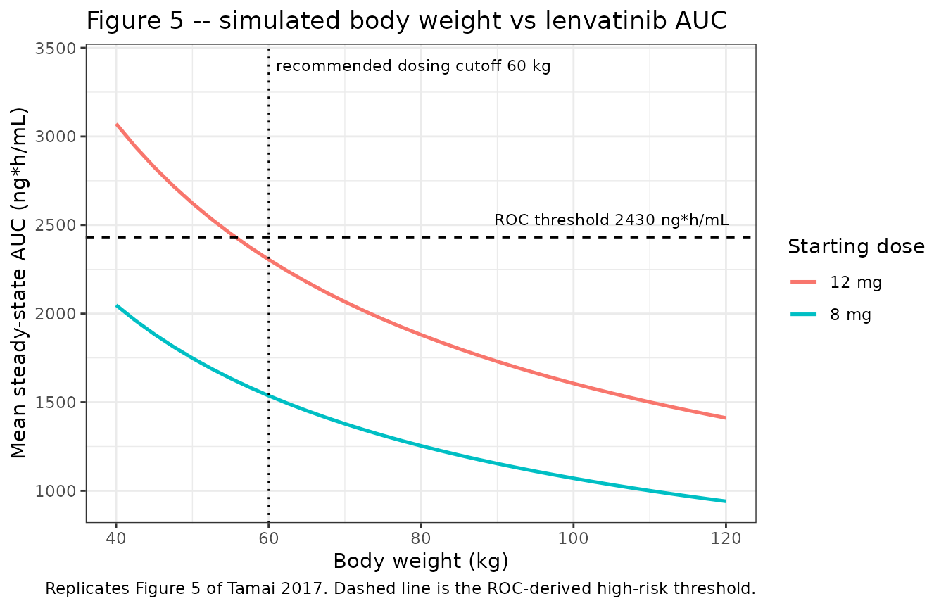
Replicates Figure 5 of Tamai 2017.
The figure carries the paper’s argument. A flat 12 mg starting dose
puts every subject below roughly 70 kg above the 2430
ng*h/mL high-risk threshold, while switching subjects under
60 kg to 8 mg moves the whole low-weight band under it and leaves the
two arms with a similar AUC span.
Figure 3 – model-predicted probability of a cycle-1 dose modification
er_probability <- function(auc) {
  ev <- data.frame(id = 1L, time = 0, amt = 0, evid = 0L, AUC_LEN = auc)
  as.data.frame(rxode2::rxSolve(
    er_mod,
    events = ev, returnType = "data.frame"
  ))$prob_teae_dosemod
}

auc_grid <- seq(1000, 5000, by = 25)
er_curve <- tibble::tibble(
  auc = auc_grid,
  prob = vapply(auc_grid, er_probability, numeric(1))
)

observed_medians <- tibble::tibble(
  auc = c(2050, 2950),
  label = c("median, no early dose modification", "median, early dose modification")
)

ggplot(er_curve, aes(auc, prob)) +
  geom_line(linewidth = 0.9) +
  geom_vline(
    data = observed_medians, aes(xintercept = auc, colour = label),
    linetype = "dashed"
  ) +
  geom_vline(xintercept = 2430, linetype = "dotted") +
  scale_y_continuous(limits = c(0, 1)) +
  labs(
    x = "Lenvatinib steady-state AUC (ng*h/mL)",
    y = "P(TEAE leading to withdrawal or dose reduction in cycle 1)",
    colour = NULL,
    title = "Figure 3 -- exposure-response for early dose modification",
    caption = "Replicates Figure 3 of Tamai 2017. Dotted line is the ROC threshold 2430 ng*h/mL."
  ) +
  theme_bw() +
  theme(legend.position = "bottom")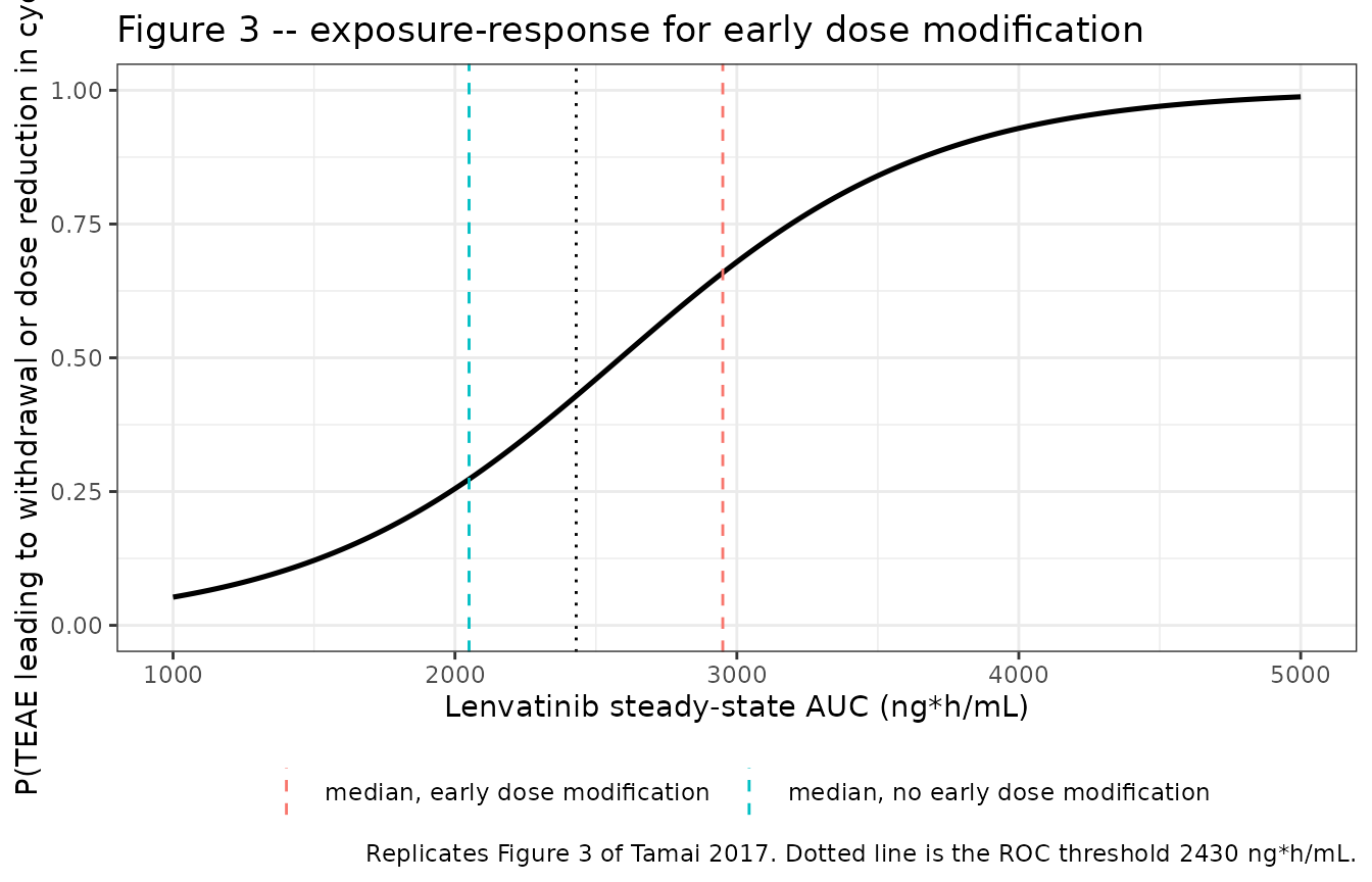
Replicates Figure 3 of Tamai 2017.
Check 4 – the exposure-response model separates the two observed groups
Tamai 2017 reports the observed AUC medians of the subjects who did and did not have an early dose modification. The fitted logistic curve must place the first group above and the second below an even chance, and the overall event rate of 46.7 percent must sit between them. These are deterministic evaluations of the model at externally reported AUC values.
p_event_group <- er_probability(2950) # median AUC, 21 subjects WITH the event
p_no_event_group <- er_probability(2050) # median AUC, 24 subjects WITHOUT
p_at_threshold <- er_probability(2430) # ROC best cutoff

round(c(
  event_group = p_event_group,
  no_event_group = p_no_event_group,
  roc_threshold = p_at_threshold
), 3)
#>    event_group no_event_group  roc_threshold
#>          0.659          0.273          0.429

stopifnot(
  p_event_group > 0.5,
  p_no_event_group < 0.5,
  # The ROC cutoff must fall between the two group medians ...
  p_at_threshold > p_no_event_group,
  p_at_threshold < p_event_group,
  # ... and near the 46.7% observed overall event rate. Realised 0.429.
  abs(p_at_threshold - 21 / 45) < 0.10
)
Check 5 – the dose recommendation the paper actually makes
The paper’s conclusion is a single arithmetic claim: a low-weight
subject on the old flat 12 mg dose sits above the 2430
ng*h/mL risk threshold, and moving to 8 mg brings them
below it while a heavy subject stays below it on 12 mg. This chains the
PK and exposure-response models exactly as the paper does.
auc_at <- function(wt, dose_mg) {
  det_ss |>
    dplyr::filter(WT == wt, dose_mg == !!dose_mg) |>
    dplyr::pull(auc_tau) * mean_factor
}

recommendation <- tibble::tibble(
  scenario = c(
    "40 kg on the old flat 12 mg",
    "40 kg on the recommended 8 mg",
    "120 kg on the recommended 12 mg"
  ),
  auc = c(auc_at(40, 12), auc_at(40, 8), auc_at(120, 12))
) |>
  dplyr::mutate(
    above_threshold = auc > 2430,
    prob_dose_mod = vapply(auc, er_probability, numeric(1))
  )

knitr::kable(
  recommendation |>
    dplyr::rename(
      "Scenario" = scenario, "Mean AUC (ng*h/mL)" = auc,
      "Above 2430 threshold" = above_threshold,
      "P(cycle-1 dose modification)" = prob_dose_mod
    ),
  digits = c(0, 0, 0, 3),
  caption = "The Tamai 2017 dose recommendation, reconstructed from the two packaged models."
)| Scenario | Mean AUC (ng*h/mL) | Above 2430 threshold | P(cycle-1 dose modification) |
|---|---|---|---|
| 40 kg on the old flat 12 mg | 3072 | TRUE | 0.707 |
| 40 kg on the recommended 8 mg | 2048 | FALSE | 0.272 |
| 120 kg on the recommended 12 mg | 1411 | FALSE | 0.105 |
stopifnot(
  recommendation$above_threshold[1], # 12 mg at 40 kg IS high risk
  !recommendation$above_threshold[2], # 8 mg at 40 kg is NOT
  !recommendation$above_threshold[3] # 12 mg at 120 kg is NOT
)
Dropping a 40 kg subject from 12 mg to 8 mg takes the predicted probability of a cycle-1 dose modification from roughly 0.71 to roughly 0.27, which is the quantitative content of the paper’s recommendation.
Steady-state concentration-time profiles
stoch_sim |>
  dplyr::filter(!is.na(Cc)) |>
  dplyr::mutate(tad = time - t_ss) |>
  dplyr::group_by(arm, tad) |>
  dplyr::summarise(
    Q05 = quantile(Cc, 0.05), Q50 = quantile(Cc, 0.50),
    Q95 = quantile(Cc, 0.95), .groups = "drop"
  ) |>
  ggplot(aes(tad, Q50)) +
  geom_ribbon(aes(ymin = Q05, ymax = Q95), alpha = 0.25) +
  geom_line() +
  facet_wrap(~arm) +
  labs(
    x = "Time after dose at steady state (h)", y = "Lenvatinib Cc (ng/mL)",
    title = "Steady-state profiles, median and 5th-95th percentile"
  ) +
  theme_bw()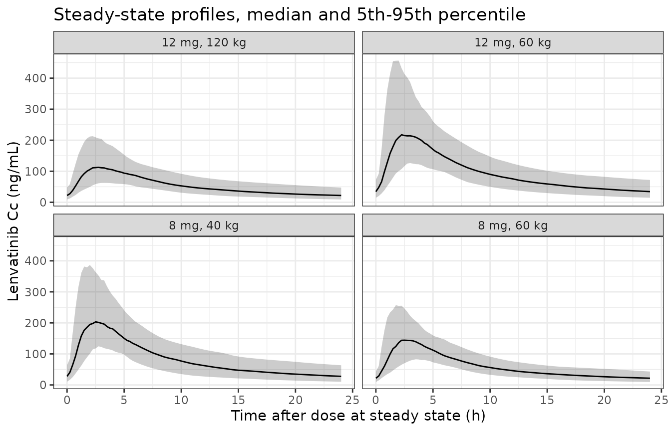
Simulated steady-state profiles by body-weight / dose corner.
PKNCA validation
sim_nca <- stoch_sim |>
  dplyr::filter(!is.na(Cc)) |>
  dplyr::select(id, time, Cc, arm) |>
  as.data.frame()

conc_obj <- PKNCA::PKNCAconc(
  sim_nca,
  formula = Cc ~ time | arm + id,
  concu = "ng/mL", timeu = "h"
)

dose_df <- stoch_events |>
  dplyr::filter(evid == 1L, time == t_ss) |>
  dplyr::select(id, time, dose_mg, arm) |>
  as.data.frame()

dose_obj <- PKNCA::PKNCAdose(
  dose_df,
  formula = dose_mg ~ time | arm + id,
  doseu = "mg"
)

intervals <- data.frame(
  start = t_ss, end = t_ss + tau,
  cmax = TRUE, tmax = TRUE, cmin = TRUE, auclast = TRUE, cav = TRUE
)

nca_res <- PKNCA::pk.nca(
  PKNCA::PKNCAdata(conc_obj, dose_obj, intervals = intervals)
)
nca_tbl <- as.data.frame(nca_res$result) |>
  dplyr::filter(PPTESTCD %in% c("cmax", "tmax", "cmin", "auclast", "cav")) |>
  dplyr::group_by(arm, PPTESTCD) |>
  dplyr::summarise(
    Median = median(PPORRES), Mean = mean(PPORRES), .groups = "drop"
  )

knitr::kable(
  nca_tbl |> dplyr::rename("Arm" = arm, "NCA parameter" = PPTESTCD),
  digits = 1,
  caption = "PKNCA steady-state results over the final 24 h dosing interval, 150 subjects per arm. Tmax is reported on the absolute clock and so includes the 480 h offset of the final dose."
)| Arm | NCA parameter | Median | Mean |
|---|---|---|---|
| 12 mg, 120 kg | auclast | 1296.0 | 1380.6 |
| 12 mg, 120 kg | cav | 54.0 | 57.5 |
| 12 mg, 120 kg | cmax | 118.6 | 126.1 |
| 12 mg, 120 kg | cmin | 21.9 | 24.9 |
| 12 mg, 120 kg | tmax | 2.8 | 2.9 |
| 12 mg, 60 kg | auclast | 2253.6 | 2396.9 |
| 12 mg, 60 kg | cav | 93.9 | 99.9 |
| 12 mg, 60 kg | cmax | 226.8 | 253.6 |
| 12 mg, 60 kg | cmin | 34.4 | 38.0 |
| 12 mg, 60 kg | tmax | 2.5 | 2.7 |
| 8 mg, 40 kg | auclast | 2045.7 | 2109.2 |
| 8 mg, 40 kg | cav | 85.2 | 87.9 |
| 8 mg, 40 kg | cmax | 212.7 | 239.1 |
| 8 mg, 40 kg | cmin | 27.7 | 30.7 |
| 8 mg, 40 kg | tmax | 2.5 | 2.6 |
| 8 mg, 60 kg | auclast | 1472.3 | 1498.8 |
| 8 mg, 60 kg | cav | 61.3 | 62.5 |
| 8 mg, 60 kg | cmax | 155.8 | 162.7 |
| 8 mg, 60 kg | cmin | 21.6 | 23.1 |
| 8 mg, 60 kg | tmax | 2.6 | 2.8 |
Comparison against published NCA
Tamai 2017 reports no observed Cmax, Tmax or half-life, so the only published NCA-scale quantities available are the four simulated steady-state AUC values of Check 2. They are means over the between-subject distribution, so the simulated side is pre-aggregated as a mean rather than left to the default median pooling.
simulated_wide <- as.data.frame(nca_res$result) |>
  dplyr::filter(PPTESTCD == "auclast") |>
  dplyr::group_by(arm) |>
  dplyr::summarise(auclast = mean(PPORRES), .groups = "drop") |>
  as.data.frame()

reference_wide <- published_corners |>
  dplyr::select(arm, auclast = auc_published) |>
  as.data.frame()

cmp <- nlmixr2lib::ncaComparisonTable(
  simulated = simulated_wide,
  reference = reference_wide,
  by = "arm",
  units = c(auclast = "ng*h/mL"),
  tolerance_pct = 20
)

knitr::kable(
  cmp,
  caption = "Simulated steady-state AUC0-tau (mean of 150 subjects per arm) against the four values Tamai 2017 reports for its Figure 5 simulation. * marks rows differing by more than 20%."
)| NCA parameter | arm | Reference | Simulated | % diff |
|---|---|---|---|---|
| AUClast (ng*h/mL) | 8 mg, 40 kg | 2050 | 2110 | +2.9% |
| AUClast (ng*h/mL) | 8 mg, 60 kg | 1540 | 1500 | -2.7% |
| AUClast (ng*h/mL) | 12 mg, 60 kg | 2310 | 2400 | +3.8% |
| AUClast (ng*h/mL) | 12 mg, 120 kg | 1410 | 1380 | -2.1% |
attr(cmp, "footnote")
#> NULL
pct <- suppressWarnings(as.numeric(gsub("[^0-9.+-]", "", cmp$`% diff`)))

# A 150-subject mean of a ~33% CV quantity carries a ~2.7% standard error, and
# the per-arm cohorts are drawn independently, so this bound admits sampling
# noise while still going red on any structural transcription error (which move
# AUC by tens of percent). The deterministic 1% gate is Check 2.
stopifnot(max(abs(pct), na.rm = TRUE) < 15)
Assumptions and deviations
-
Absorption is encoded as sequential
zero-order-then-first-order, not as a parallel dose split.
Tamai 2017 Methods describe “simultaneous first- and 0-order absorption”
and Table 2 reports exactly two absorption parameters,
KaandD1, plusF1.D1andF1are the NONMEM duration and bioavailability of dosing compartment 1, which is the depot, so the whole dose enters the depot, is released into it overD1hours at zero order, and leaves it first-order atKa– both processes acting at once, which is what makes the paper’s word “simultaneous” apt. A genuinely parallel model, with part of the dose going first-order and part zero-order, requires a split fraction, and no such parameter is reported anywhere in Tamai 2017. The sequential encoding is therefore the only one that can be built without inventing a number. This differs from the siblingGupta_2016_lenvatinib, which implements a parallel 50:50 split intodepotandcentraland states in its own model file that the fraction is an undisclosed assumption; the two lenvatinib popPK entries consequently disagree on absorption structure. The disagreement does not touch AUC, which depends only on dose and CL/F, so every check in this vignette is unaffected; it does change Tmax and Cmax. - Mammillary, not catenary, three-compartment disposition. Tamai 2017 Methods list “apparent volume of peripheral compartments (V2/F and V3/F), intercompartmental clearance between V2 and V3 (Q2/F and Q3/F)” in parallel construction – one intercompartmental clearance per peripheral compartment, both exchanging with central. The Table 2 abbreviation list renumbers these to Q1 and Q2 and glosses Q2 as “intercompartment clearance between V2 and V3”, which read literally would be a catenary chain. That gloss is a carry-over slip from the Methods sentence: under it, the Methods clause would assign two parameters to a single V2-V3 link. The mammillary reading matches the predecessor model of the same drug and sponsor and NONMEM’s ADVAN12, and is what is encoded here.
-
Interindividual variances are read as the squared
%CV. Table 2 footnote a defines the printed column as “the
square root of the variance x 100”, so
omega^2 = (%CV/100)^2. The siblingGupta_2016_lenvatinibinstead applies the log-normal conversionlog(CV^2 + 1)to its own table. Check 2 supports the reading used here, though only weakly – the two readings differ by 0.26 percent on the mean-AUC factor, against a 0.21 percent achieved residual, so the footnote rather than the arithmetic is the decisive evidence. -
The alkaline phosphatase ULN is not from the paper.
Tamai 2017 enters ALP only as an above-/at-or-below-ULN indicator and
never prints the numeric cutoff.
alp_uln <- 120U/L inmodel()is a representative adult value carried fromGupta_2016_lenvatinib; it is the only non-source-derived number in the PK model file. Downstream users should supply a pre-binarised ALP column or edit the cutoff to their laboratory’s ULN. All checks in this vignette are run at ALP = 81.5 U/L, the Table 1 median, which is below any plausible adult ULN, so none depends on the specific value chosen. - The residual error model is simplified from three strata to one. Tamai 2017 fits a combined proportional-plus-additive error for time after dose at or below 2 h (44.8 percent CV proportional plus 7.35 ng/mL additive) and separate proportional errors for the clinical pharmacology studies (17.3 percent CV) and the cancer-patient studies (30.2 percent CV). rxode2 cannot switch a residual model on time after dose. The library model carries the cancer-patient proportional term – the stratum applying to the HCC population the paper is about – together with the additive term. The two unused proportional arms are quoted here so a user refitting can restore them.
-
The exposure-response model’s residual is a
placeholder. Tamai 2017 fits a logistic regression with a
Bernoulli likelihood, which estimates no residual error.
addSd_prob_teae_dosemod <- fixed(0.001)exists only so rxode2 has an error model to attach to the typical-value probability and is not a published quantity. It follows the convention of the other landmark exposure-response models in this package. -
The exposure-response model retains no covariate, and that
is a published result. Demographics, liver-function markers,
baseline platelet count, ECOG performance status, Child-Pugh class,
hepatitis B or C aetiology, portal-vein involvement, prior systemic
chemotherapy, prior antihypertensive therapy and prior surgery were all
screened and none influenced the relationship. They are recorded in the
model file’s
covariatesDataExcludedrather than encoded asfixed(0)coefficients, because no coefficient was ever estimated. The same applies to steady-state minimum concentration, the rival exposure metric that AUC beat. - Body weight was screened on the exposure-response relationship and not retained. This is not a claim that weight is irrelevant to toxicity – it is central to the paper – but that it acts entirely through exposure, via the CL/F weight term of the PK model, and adds nothing once AUC is in the logit. Check 5 shows the chain working in exactly that direction.
- No exposure-efficacy relationship is modelled. Tamai 2017 evaluated time to progression against AUC tertiles by Kaplan-Meier and found none (Figure 6), so there is no efficacy model to extract. That null result is what makes a lower starting dose acceptable to the authors.
- Virtual covariate distributions. Original study 202 data are not public. The cohorts here fix body weight at the paper’s own quoted values rather than sampling a distribution, because every published number this vignette checks against is quoted at a specific weight.