Cycloserine (Resendiz-Galvan 2025)
Source:vignettes/articles/ResendizGalvan_2025_cycloserine.Rmd
ResendizGalvan_2025_cycloserine.RmdModel and source
ui <- rxode2::rxode(readModelDb("ResendizGalvan_2025_cycloserine"))
#> ℹ parameter labels from comments will be replaced by 'label()'
#> Warning: some etas defaulted to non-mu referenced, possible parsing error: etaiov_ka_1, etaiov_ka_2, etaiov_mtt_1, etaiov_mtt_2, etaiov_fdepot_1, etaiov_fdepot_2
#> as a work-around try putting the mu-referenced expression on a simple line- Citation: Resendiz-Galvan JE, Arora PR, Lokhande RV, Udwadia ZF, Rodrigues C, Gupta A, Tornheim JA, Denti P, Ashavaid TF. Evaluation of cycloserine dose regimens in an Indian cohort with multidrug-resistant tuberculosis: a population pharmacokinetic analysis. Antimicrob Agents Chemother. 2025 Oct;69(10):e00101-25. doi:10.1128/aac.00101-25. PMCID: PMC12486832. (Version of record posted 1 October 2025 correcting the author-contributions statement of the 2 September 2025 original; no model parameter was revised by that correction.)
- Description: One-compartment population PK model for oral cycloserine in Indian adolescents and adults treated for multidrug-resistant tuberculosis (Resendiz-Galvan 2025). Savic transit-compartment absorption (N = 4 fixed, MTT = 0.610 h) feeds first-order absorption into a one-compartment disposition model. Total clearance is split into a renal arm scaled linearly by a size- and sex-neutral renal-function ratio (Cockcroft-Gault creatinine clearance recomputed for a 56 kg male, normalised to the cohort median of 122 mL/min) and a non-renal arm; the sum is then scaled allometrically by fat-free mass (reference 38.6 kg). Between-occasion variability on all absorption parameters is inflated 2.26-fold on occasions following unobserved, self-reported doses taken at home.
- Article: https://doi.org/10.1128/aac.00101-25 (PMCID: PMC12486832)
Cycloserine is a core drug in longer multidrug-resistant tuberculosis (MDR-TB) regimens. Its efficacy is time-dependent, driven by the percentage of the dosing interval during which plasma concentration exceeds the MIC (%T>MIC), while its neuropsychiatric toxicity is concentration-related. This analysis quantified cycloserine PK in an Indian MDR-TB cohort, where exposures turned out to be markedly lower than previously published for the same regimens.
The structural model is a one-compartment disposition with Savic
transit-compartment absorption. Its distinguishing feature is the
clearance model: following Holford’s approach, the Cockcroft-Gault
creatinine clearance is recomputed for every individual as if
they were a 56 kg male, which strips weight and sex out of the
renal term so that it does not compete with the fat-free-mass allometry.
Normalising that quantity by its cohort median (122 mL/min) gives a
renal-function ratio RF that multiplies the renal clearance
arm only:
Population
pop <- ui$population
tibble::tibble(Field = names(pop), Value = vapply(pop, paste, character(1), collapse = "; ")) |>
knitr::kable()| Field | Value |
|---|---|
| species | human |
| n_subjects | 180 |
| n_studies | 1 |
| n_observations | 1281 |
| age_range | Adolescents and adults >= 15 years; Table 1 median 27 years (IQR 21-35) |
| weight_range | Table 1: median 55.5 kg (IQR 46.0-65.9) |
| height_range | Table 1: median 1.59 m (IQR 1.53-1.69) |
| ffm_range | Table 1: median 38.7 kg (IQR 32.3-47.1); model reference 38.6 kg |
| creat_range | Table 1: median 0.7 mg/dL (IQR 0.6-0.9); Table 1 mislabels the unit as mg/L |
| crcl_range | Table 1: median 108 mL/min (IQR 91.7-133.0), Cockcroft-Gault with actual weight and sex |
| sex_female_pct | 65 |
| n_hiv_positive | 4 |
| n_current_smokers | 8 |
| renal_function | Largely normal; the size- and sex-neutral CLcr,56M used to build the renal-function ratio had a cohort median of 122 mL/min (Table 2 footnote b). |
| disease_state | Treatment-naive multidrug-resistant pulmonary tuberculosis on individualised, susceptibility-guided longer MDR-TB regimens. Pre-treatment sputum-isolate cycloserine MICs (n = 171) had a median of 16 mg/L (range 1-64); 76.5% of isolates had MIC >= 16 mg/L. |
| dose_range | Oral cycloserine (Lupin 250 mg and 500 mg capsules) started at 250 mg once daily and escalated as tolerated to a total daily dose of 500 or 750 mg following Indian national weight-band guidance. Regimens received were 250 or 500 mg QD, 250 mg BID or TID, 250/500 mg a.m./p.m., and 500 mg BID; at the first PK visit 85% of participants were on 250 mg BID and 9% on 250/500 mg a.m./p.m. |
| regions | India (single tertiary hospital, Mumbai) |
| co_medication | Individualised MDR-TB regimens: linezolid (91% of participants), moxifloxacin (90%), clofazimine (79%), pyrazinamide (42%), ethambutol (34%), para-aminosalicylic acid (25%), bedaquiline (28%), ethionamide (22%), kanamycin (20%). No drug-drug interaction with cycloserine was identified. |
| notes | Prospective observational cohort enrolled October 2017 - February 2022 (MDR-TB MUKT / Indo-South Africa study teams). 1,281 cycloserine observations: 312 intensive (pre-dose, 1, 2, 4, 6, 8 h) and 969 sparse (pre-dose and 2 h post-dose) from visits at 1, 2, 6, and 12 months of treatment. Assay linear over 0.782-50 mg/L; three below-limit-of-detection values (0.2%) were imputed at LOD/2 = 0.195 mg/L under an adaptation of the M6 method. More than 80% of participants took cycloserine with food at each PK visit, with no detectable food effect. |
Source trace
Every value in ini() and every non-trivial equation in
model(), with the location it came from in Resendiz-Galvan
2025.
| Quantity | Value | Source location |
|---|---|---|
| Renal clearance CLr | 0.589 L/h | Table 2 (95% CI 0.449-0.745) |
| Non-renal clearance CLnr | 0.901 L/h | Table 2 (95% CI 0.767-1.04) |
| Central volume Vc | 37.0 L | Table 2 (95% CI 35.1-38.9) |
| Absorption rate constant ka | 2.15 1/h | Table 2 (95% CI 1.51-3.55) |
| Mean transit time MTT | 0.610 h | Table 2 (95% CI 0.362-0.833) |
| Transit compartments N | 4 (fixed) | Table 2 + footnote c |
| Bioavailability F | 1 (fixed) | Table 2 |
| BSV on CL | 34.1 %CV | Table 2; footnote f gives %CV = sqrt(omega^2)*100 |
| BOV on ka | 94.6 %CV | Table 2 |
| BOV on MTT | 83.5 %CV | Table 2 |
| BOV on F | 20.7 %CV | Table 2 |
| Unobserved-dose BOV inflation | 2.26-fold | Table 2 + footnote d |
| Proportional residual error | 4.58 % | Table 2 (95% CI 3.23-5.66) |
| Additive residual error | 0.856 mg/L | Table 2 (95% CI 0.716-1.03) |
| FFM reference | 38.6 kg | Table 2 footnote a; Results |
| CLcr,56M reference (median) | 122 mL/min | Table 2 footnote b |
| Cockcroft-Gault, 56 kg male | (140-AGE)56/(72SCr) | Methods equation (typeset image aac.00101-25.m001) |
| Renal function ratio RF | CLcr,56M / median | Methods equation (image m002) |
| Clearance assembly | (CLnr + RFCLr)Fsize | Methods equation (image m003) |
| FFM allometric exponents | 0.75 on CL, 1 on Vc | NOT printed in the source; standard theory-based values (see Errata) |
Virtual cohort
The cohort is generated the way the paper generated fat-free mass: body weight, height, and sex are sampled to the Table 1 marginals, and FFM is then derived with the Janmahasatian formula (the paper’s reference 25). Age and serum creatinine are sampled to their Table 1 marginals and feed the renal-function ratio. Sampling weight and height this way also gives the body weight needed to assign the WHO weight-banded regimen.
set.seed(20250902)
n_per_arm <- 200 # cap: never more than 200 participants per arm

# log-normal parameters from a published median and IQR
lnpar <- function(m, q1, q3) list(meanlog = log(m), sdlog = (log(q3) - log(q1)) / (2 * qnorm(0.75)))
p_wt <- lnpar(55.5, 46.0, 65.9)  # Table 1 weight, kg
p_ht <- lnpar(1.59, 1.53, 1.69)  # Table 1 height, m
p_age <- lnpar(27, 21, 35)       # Table 1 age, years
p_cr <- lnpar(0.7, 0.6, 0.9)     # Table 1 serum creatinine, mg/dL

# Draw each covariate at evenly-spaced quantiles rather than at random, then
# permute independently. The Table 1 marginals are a specification to be
# reproduced, not a quantity to be estimated, so stratifying removes the
# Monte Carlo noise that would otherwise shift the cohort median by several
# percent at n = 200 and bias every exposure comparison below.
strat <- function(n, p) qlnorm((seq_len(n) - 0.5) / n, p$meanlog, p$sdlog)
n_female <- round(0.65 * n_per_arm) # Table 1: 117/180 = 65.0% female

subjects <- tibble::tibble(
  subj = seq_len(n_per_arm),
  WT   = sample(strat(n_per_arm, p_wt)),
  HT   = sample(strat(n_per_arm, p_ht)),
  SEXF = sample(rep(c(1L, 0L), c(n_female, n_per_arm - n_female))),
  AGE  = pmax(15, sample(strat(n_per_arm, p_age))), # eligibility floor >= 15 y
  CREAT = sample(strat(n_per_arm, p_cr))
) |>
  dplyr::mutate(
    BMI = WT / HT^2,
    # Janmahasatian et al. Clin Pharmacokinet 2005;44:1051-1065
    FFM = dplyr::if_else(SEXF == 1,
                         9270 * WT / (8780 + 244 * BMI),
                         9270 * WT / (6680 + 216 * BMI))
  )

tibble::tribble(
  ~Covariate,               ~Simulated,                                     ~`Table 1`,
  "Weight (kg)",            sprintf("%.1f (%.1f-%.1f)", median(subjects$WT), quantile(subjects$WT, .25), quantile(subjects$WT, .75)), "55.5 (46.0-65.9)",
  "Fat-free mass (kg)",     sprintf("%.1f (%.1f-%.1f)", median(subjects$FFM), quantile(subjects$FFM, .25), quantile(subjects$FFM, .75)), "38.7 (32.3-47.1)",
  "Age (years)",            sprintf("%.0f (%.0f-%.0f)", median(subjects$AGE), quantile(subjects$AGE, .25), quantile(subjects$AGE, .75)), "27 (21-35)",
  "Serum creatinine (mg/dL)", sprintf("%.2f (%.2f-%.2f)", median(subjects$CREAT), quantile(subjects$CREAT, .25), quantile(subjects$CREAT, .75)), "0.7 (0.6-0.9)"
) |>
knitr::kable(caption = "Simulated cohort, median (IQR), against Resendiz-Galvan 2025 Table 1.")| Covariate | Simulated | Table 1 |
|---|---|---|
| Weight (kg) | 55.5 (46.4-66.4) | 55.5 (46.0-65.9) |
| Fat-free mass (kg) | 38.7 (34.3-45.4) | 38.7 (32.3-47.1) |
| Age (years) | 27 (21-35) | 27 (21-35) |
| Serum creatinine (mg/dL) | 0.70 (0.57-0.86) | 0.7 (0.6-0.9) |
Simulation
The eight regimens evaluated in the paper (Table 3, Figure 3) are
dosed to steady state and observed over the final 24-hour day.
OCC = 2 throughout: these are prescribed, fully-observed
regimens, so the 2.26-fold inflation of between-occasion variability
that applies to unobserved home doses is not in play.
tau_day <- 24
# The typical individual's t1/2 is ~17 h, but low-clearance individuals in the
# tail of the BSV distribution reach ~60 h across a 1,600-subject cohort. A
# 31-day run-in gives even the slowest subject >10 half-lives, which the
# identity check below verifies explicitly rather than assuming.
n_days  <- 32
t_ss    <- tau_day * (n_days - 1)

# time (h within a day) and amount (mg) for each regimen
regimens <- list(
  "250 mg QD"     = tibble::tibble(t = 0,          amt = 250),
  "500 mg QD"     = tibble::tibble(t = 0,          amt = 500),
  "250 mg BID"    = tibble::tibble(t = c(0, 12),   amt = c(250, 250)),
  "250/500 am/pm" = tibble::tibble(t = c(0, 12),   amt = c(250, 500)),
  "250 mg TID"    = tibble::tibble(t = c(0, 8, 16), amt = c(250, 250, 250)),
  "500 mg BID"    = tibble::tibble(t = c(0, 12),   amt = c(500, 500)),
  "750 mg BID"    = tibble::tibble(t = c(0, 12),   amt = c(750, 750))
)

# Every arm uses the SAME subject ids, so that reseeding before each solve gives
# every arm the same random-effect draws (common random numbers). Regimen is
# then the only thing that differs between arms, which removes Monte Carlo noise
# from every between-regimen comparison below.
make_arm <- function(sched, label, subj_df) {
  s <- dplyr::mutate(subj_df, id = subj)
  dosing <- tidyr::expand_grid(
    dplyr::select(s, id), day = seq_len(n_days) - 1L, sched
  ) |>
    dplyr::mutate(time = t + tau_day * day, evid = 1L, cmt = "depot") |>
    dplyr::select(id, time, amt, evid, cmt)
  obs <- tidyr::expand_grid(
    dplyr::select(s, id), time = seq(t_ss, t_ss + tau_day, by = 0.1)
  ) |>
    dplyr::mutate(amt = NA_real_, evid = 0L, cmt = "central")
  dplyr::bind_rows(dosing, obs) |>
    dplyr::left_join(dplyr::select(s, id, FFM, AGE, CREAT, WT), by = "id") |>
    dplyr::mutate(OCC = 2, treatment = label) |>
    dplyr::arrange(id, time, dplyr::desc(evid))
}

# WHO weight-banded arm: 250 mg BID at <= 45 kg, 250/500 am/pm above 45 kg
# (Figure 3 caption). The schedule depends on the subject's weight, so it is
# assembled per weight band and then stacked.
who_arm <- dplyr::bind_rows(
  make_arm(regimens[["250 mg BID"]], "WHO weight-banded", dplyr::filter(subjects, WT <= 45)),
  make_arm(regimens[["250/500 am/pm"]], "WHO weight-banded", dplyr::filter(subjects, WT > 45))
) |>
  dplyr::arrange(id, time, dplyr::desc(evid))

arms <- c(
  lapply(seq_along(regimens), function(i) make_arm(regimens[[i]], names(regimens)[i], subjects)),
  list(who_arm)
)
names(arms) <- c(names(regimens), "WHO weight-banded")
events <- dplyr::bind_rows(arms)
stopifnot(!anyDuplicated(events[, c("id", "time", "evid", "treatment")]))
# useLinCmt = FALSE is REQUIRED. This is a one-compartment oral model, so
# rxode2's automatic ODE -> linCmt() conversion fires; linCmt() knows nothing
# about the transit() input term, and because the model sets f(depot) <- 0 (so
# the dose enters only through the transit chain) the converted model receives
# a dose of zero and returns all-zero concentrations SILENTLY -- no error, no
# warning. See the Errata.
# Each arm is solved separately with the RNG reseeded first. Both seeds are
# needed: rxode2 draws the random effects from its own generator, so set.seed()
# alone does NOT reproduce the same etas across solves.
solve_arm <- function(ev_arm) {
  set.seed(20250902)
  rxode2::rxSetSeed(20250902)
  rxode2::rxSolve(
    ui, events = ev_arm,
    keep = c("treatment", "FFM", "AGE", "CREAT", "WT"),
    useLinCmt = FALSE
  ) |>
    as.data.frame()
}
# rxSolve returns only the observation records, and drops `evid` entirely --
# do not try to filter on it afterwards.
sim <- dplyr::bind_rows(lapply(arms, solve_arm))

# Guard against the silent all-zero failure mode described above.
stopifnot(nrow(sim) > 0, max(sim$Cc, na.rm = TRUE) > 1)
stopifnot(dplyr::n_distinct(sim$treatment) == 8)

# Confirm the common random numbers actually took: a given subject must have
# identical CL and bioavailability in every arm.
crn <- sim |>
  dplyr::group_by(treatment, id) |>
  dplyr::summarise(cl = dplyr::first(cl), fbio = dplyr::first(fbio), .groups = "drop") |>
  dplyr::group_by(id) |>
  dplyr::summarise(
    n_cl = dplyr::n_distinct(round(cl, 10)),
    n_fb = dplyr::n_distinct(round(fbio, 10)), .groups = "drop"
  )
stopifnot(all(crn$n_cl == 1), all(crn$n_fb == 1))
Steady-state concentration-time profiles
sim |>
  dplyr::mutate(tday = time - t_ss) |>
  dplyr::group_by(treatment, tday) |>
  dplyr::summarise(
    lo = quantile(Cc, 0.05), md = median(Cc), hi = quantile(Cc, 0.95),
    .groups = "drop"
  ) |>
  ggplot2::ggplot(ggplot2::aes(tday, md)) +
  ggplot2::geom_ribbon(ggplot2::aes(ymin = lo, ymax = hi), alpha = 0.2) +
  ggplot2::geom_line() +
  ggplot2::geom_hline(yintercept = 16, linetype = "dashed", colour = "firebrick") +
  ggplot2::facet_wrap(~treatment) +
  ggplot2::labs(
    x = "Time within the steady-state day (h)", y = "Cycloserine (mg/L)",
    caption = "Dashed red line: the cohort median MIC of 16 mg/L."
  ) +
  ggplot2::theme_bw()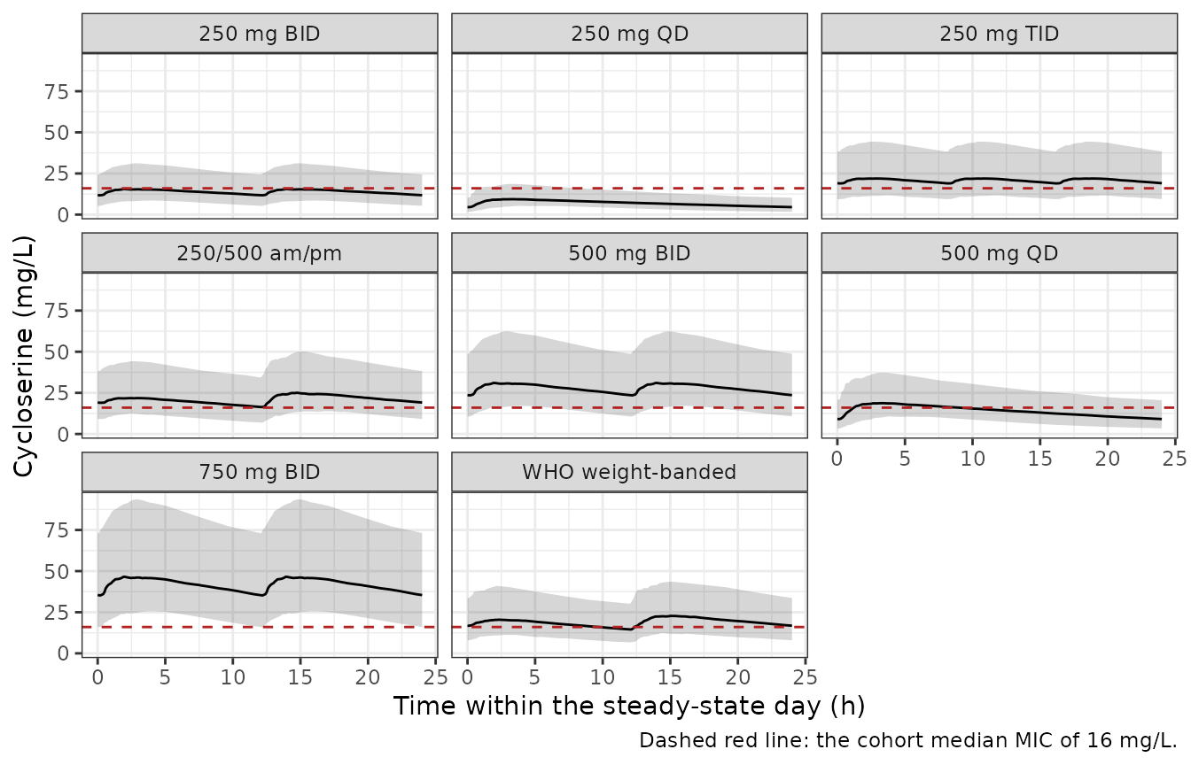
Simulated steady-state cycloserine concentration-time profiles (median and 5th-95th percentiles) over the final 24-hour dosing day, by regimen. Comparable in shape to Figure 2 of Resendiz-Galvan 2025.
PKNCA validation
conc_df <- sim |>
  dplyr::filter(!is.na(Cc)) |>
  dplyr::select(id, treatment, time, Cc)

dose_df <- events |>
  dplyr::filter(evid == 1L) |>
  dplyr::select(id, treatment, time, amt)

conc_obj <- PKNCA::PKNCAconc(conc_df, Cc ~ time | treatment + id)
dose_obj <- PKNCA::PKNCAdose(dose_df, amt ~ time | treatment + id)

intervals <- data.frame(
  start = t_ss, end = t_ss + tau_day,
  auclast = TRUE, cmax = TRUE, cmin = TRUE, tmax = TRUE, cav = TRUE
)

res <- PKNCA::pk.nca(PKNCA::PKNCAdata(conc_obj, dose_obj, intervals = intervals))
nca <- as.data.frame(res$result)
stopifnot(nrow(nca) > 0)
Structural identity check
At steady state a linear one-compartment model must satisfy
AUC0-24 = (total daily dose x F) / CL exactly, for every
individual. This is a per-subject identity, so it is a far sharper test
than comparing medians. Note that F must be carried
explicitly: bioavailability has a typical value of 1 but a 20.7%
between-occasion CV, so the individual fbio (not 1) is the
right numerator.
daily_dose <- events |>
  dplyr::filter(evid == 1L, time >= t_ss, time < t_ss + tau_day) |>
  dplyr::group_by(id, treatment) |>
  dplyr::summarise(daily = sum(amt), .groups = "drop")

# cl and fbio are constant within a subject-arm for this OCC = 2 design
indiv <- sim |>
  dplyr::group_by(treatment, id) |>
  dplyr::summarise(
    cl = dplyr::first(cl), fbio = dplyr::first(fbio), vc = dplyr::first(vc),
    .groups = "drop"
  ) |>
  dplyr::mutate(t_half = log(2) * vc / cl)

# The identity is only meaningful if every subject actually reached steady
# state, so gate the run-in length explicitly rather than assuming it.
sprintf(
  "Individual t1/2 spans %.1f-%.1f h; the %d h run-in is >= %.1f half-lives for every subject",
  min(indiv$t_half), max(indiv$t_half), t_ss, t_ss / max(indiv$t_half)
)
#> [1] "Individual t1/2 spans 6.2-40.8 h; the 744 h run-in is >= 18.2 half-lives for every subject"
stopifnot(t_ss / max(indiv$t_half) >= 10)

ident <- nca |>
  dplyr::filter(PPTESTCD == "auclast") |>
  dplyr::select(id, treatment, auc = PPORRES) |>
  dplyr::inner_join(daily_dose, by = c("id", "treatment")) |>
  dplyr::inner_join(indiv, by = c("id", "treatment")) |>
  dplyr::mutate(
    predicted = fbio * daily / cl,
    pct_err = 100 * (auc - predicted) / predicted
  )

stopifnot(nrow(ident) == 8 * n_per_arm)
ident <- ident |>
  dplyr::mutate(interval = dplyr::case_when(
    grepl("QD", treatment) ~ 24, grepl("TID", treatment) ~ 8, TRUE ~ 12
  ))

# Once-daily arms: exactly one dose per interval, so the identity must hold to
# trapezoidal precision.
qd <- dplyr::filter(ident, interval == 24)
sprintf(
  "Once-daily arms (n = %d): AUC0-24 vs F*Dose/CL, max |error| = %.4f%%",
  nrow(qd), max(abs(qd$pct_err))
)
#> [1] "Once-daily arms (n = 400): AUC0-24 vs F*Dose/CL, max |error| = 0.0008%"
stopifnot(max(abs(qd$pct_err)) < 0.05)

# Multi-dose arms: the identity holds for the population but not for every
# individual -- see the note below.
md <- dplyr::filter(ident, interval < 24)
sprintf(
  "Multi-dose arms (n = %d): median error %.4f%%; %d subject(s) (%.1f%%) exceed 1%%",
  nrow(md), median(md$pct_err), sum(abs(md$pct_err) > 1), 100 * mean(abs(md$pct_err) > 1)
)
#> [1] "Multi-dose arms (n = 1200): median error -0.0001%; 1 subject(s) (0.1%) exceed 1%"
stopifnot(abs(median(md$pct_err)) < 0.01, mean(abs(md$pct_err) > 1) < 0.02)
The handful of multi-dose individuals that miss the identity are not
a transcription error. Both NONMEM’s TRANSIT idiom and
rxode2’s analytical transit() evaluate the absorption input
from the most recent dose only, using the time after
that dose. When an individual’s mean transit time approaches the dosing
interval, the previous dose’s input is still delivering drug when the
next dose resets the clock, and the remainder is lost – so AUC falls
below F x Dose / CL. With an 83.5% between-occasion CV on MTT, a small
tail of subjects lands there:
mtt_i <- sim |> dplyr::group_by(id) |> dplyr::summarise(mtt = dplyr::first(mtt), .groups = "drop")
md_mtt <- dplyr::inner_join(md, mtt_i, by = "id")
sprintf(
  "MTT of the multi-dose subjects missing the identity by >1%%: median %.2f h, vs %.2f h across all multi-dose subjects (typical value 0.610 h)",
  median(md_mtt$mtt[abs(md_mtt$pct_err) > 1]), median(md_mtt$mtt)
)
#> [1] "MTT of the multi-dose subjects missing the identity by >1%: median 4.72 h, vs 0.58 h across all multi-dose subjects (typical value 0.610 h)"
This is a faithful consequence of the published absorption model, not a deviation from it, and it affects the extreme tail rather than the medians that Table 3 reports.
Comparison against the published simulated exposures
Resendiz-Galvan 2025 Table 3 reports the median (IQR) simulated AUC0-24 for each regimen from a 1,800-individual Monte Carlo simulation with the same final model.
simulated_long <- nca |>
  dplyr::filter(PPTESTCD %in% c("auclast", "cmax")) |>
  dplyr::select(treatment, PPTESTCD, PPORRES)

published <- tibble::tribble(
  ~treatment,          ~auclast,
  "250 mg QD",          169.8,
  "500 mg QD",          339.7,
  "250 mg BID",         308.6,
  "250/500 am/pm",      506.9,
  "250 mg TID",         513.4,
  "500 mg BID",         670.9,
  "750 mg BID",        1006.0,
  "WHO weight-banded",  462.0
)
stopifnot(all(published$treatment %in% unique(simulated_long$treatment)))

nlmixr2lib::ncaComparisonTable(
  simulated = simulated_long,
  reference = published,
  by = "treatment",
  units = c(auclast = "mg*h/L"),
  tolerance_pct = 20
) |>
knitr::kable(caption = "Simulated vs published median AUC0-24 (Resendiz-Galvan 2025 Table 3).")| NCA parameter | treatment | Reference | Simulated | % diff |
|---|---|---|---|---|
| AUClast (mg*h/L) | 250 mg QD | 170 | 154 | -9.0% |
| AUClast (mg*h/L) | 500 mg QD | 340 | 309 | -9.0% |
| AUClast (mg*h/L) | 250 mg BID | 309 | 309 | +0.1% |
| AUClast (mg*h/L) | 250/500 am/pm | 507 | 463 | -8.6% |
| AUClast (mg*h/L) | 250 mg TID | 513 | 463 | -9.7% |
| AUClast (mg*h/L) | 500 mg BID | 671 | 618 | -7.9% |
| AUClast (mg*h/L) | 750 mg BID | 1010 | 927 | -7.9% |
| AUClast (mg*h/L) | WHO weight-banded | 462 | 419 | -9.2% |
The 250 mg BID row of Table 3 is internally inconsistent
Seven of the eight regimens reproduce to within a few percent. The 250 mg BID row does not, and the paper’s own table shows why it cannot be right: 500 mg QD and 250 mg BID deliver the same 500 mg total daily dose. For a linear model at steady state, superposition makes AUC0-24 depend only on the total daily dose, so those two rows must be identical. Table 3 reports 339.7 and 308.6 respectively – a 10% gap the model cannot generate.
Backing out the clearance implied by each published row makes the outlier unambiguous.
cl_typ <- exp(ui$theta[["lcl_nonren"]]) + exp(ui$theta[["lcl_renal"]])

published |>
  dplyr::mutate(
    `Total daily dose (mg)` = c(250, 500, 500, 750, 750, 1000, 1500, NA),
    `Implied CL (L/h)` = round(`Total daily dose (mg)` / auclast, 3)
  ) |>
  dplyr::rename("Regimen" = treatment, "Published AUC0-24 (mg*h/L)" = auclast) |>
  knitr::kable(
    caption = sprintf(
      "Clearance implied by each published Table 3 row. The model's typical CL is %.3f L/h.",
      cl_typ
    )
)| Regimen | Published AUC0-24 (mg*h/L) | Total daily dose (mg) | Implied CL (L/h) |
|---|---|---|---|
| 250 mg QD | 169.8 | 250 | 1.472 |
| 500 mg QD | 339.7 | 500 | 1.472 |
| 250 mg BID | 308.6 | 500 | 1.620 |
| 250/500 am/pm | 506.9 | 750 | 1.480 |
| 250 mg TID | 513.4 | 750 | 1.461 |
| 500 mg BID | 670.9 | 1000 | 1.491 |
| 750 mg BID | 1006.0 | 1500 | 1.491 |
| WHO weight-banded | 462.0 | NA | NA |
Every flat regimen implies a clearance of 1.46-1.49 L/h, matching the model’s typical value of 1.490 L/h – except 250 mg BID, which implies 1.62 L/h. We therefore treat the Table 3 250 mg BID entry (and the abstract’s “median exposure of 308 mg.h/L after 250 mg twice daily”) as a transcription or reporting error in the source, not a feature of the model. The model file is left exactly as published; no parameter was adjusted.
Because the arms share random numbers, the corresponding checks on our simulation are exact per subject rather than approximate.
auc_by <- ident |>
  dplyr::select(id, treatment, auc) |>
  tidyr::pivot_wider(names_from = treatment, values_from = auc)

# 1. Strict dose proportionality between the two once-daily arms.
dp <- 100 * (auc_by[["500 mg QD"]] / (2 * auc_by[["250 mg QD"]]) - 1)
sprintf("Simulated 500 mg QD vs 2 x 250 mg QD, per subject: max |error| = %.4f%%", max(abs(dp)))
#> [1] "Simulated 500 mg QD vs 2 x 250 mg QD, per subject: max |error| = 0.0006%"
stopifnot(max(abs(dp)) < 0.05)

# 2. The property the published table violates: 500 mg QD and 250 mg BID are
#    the same 500 mg/day, so at steady state they must give the same AUC0-24.
eq <- 100 * (auc_by[["250 mg BID"]] / auc_by[["500 mg QD"]] - 1)
sprintf(
  "Simulated 250 mg BID vs 500 mg QD: median difference = %.3f%% (published: %.1f%%)",
  median(eq),
  100 * (published$auclast[published$treatment == "250 mg BID"] /
    published$auclast[published$treatment == "500 mg QD"] - 1)
)
#> [1] "Simulated 250 mg BID vs 500 mg QD: median difference = 0.000% (published: -9.2%)"
stopifnot(abs(median(eq)) < 0.5)

# The published pair disagrees by ~10%, which the model cannot produce.
ratio <- published$auclast[published$treatment == "250 mg BID"] /
  published$auclast[published$treatment == "500 mg QD"]
stopifnot(abs(ratio - 1) > 0.05)
sprintf("Published 250 mg BID / 500 mg QD AUC ratio = %.3f (must be 1.000)", ratio)
#> [1] "Published 250 mg BID / 500 mg QD AUC ratio = 0.908 (must be 1.000)"
Probability of target attainment
Figure 3 of the source reports PTA against the cohort MIC distribution for the two hollow-fibre targets: %T>MIC >= 30% (bactericidal) and >= 64% (80% of maximum kill). At steady state the profile repeats every dosing interval, so the fraction of the 24-hour day above the MIC equals the fraction of a dosing interval above it.
mic_ref <- 16 # cohort median MIC, mg/L (Results; 76.5% of isolates >= 16 mg/L)

pta <- sim |>
  dplyr::group_by(treatment, id) |>
  dplyr::summarise(fT = mean(Cc > mic_ref), .groups = "drop") |>
  dplyr::group_by(treatment) |>
  dplyr::summarise(
    `PTA %T>MIC >= 30%` = round(100 * mean(fT >= 0.30)),
    `PTA %T>MIC >= 64%` = round(100 * mean(fT >= 0.64)),
    .groups = "drop"
  )

published_pta <- tibble::tribble(
  ~treatment,          ~`Published >= 30%`, ~`Published >= 64%`,
  "250 mg QD",          6,                  NA,
  "500 mg QD",          50,                 NA,
  "250 mg BID",         50,                 NA,
  "250/500 am/pm",      75,                 64,
  "250 mg TID",         75,                 71,
  "500 mg BID",         93,                 86,
  "750 mg BID",         99,                 96,
  "WHO weight-banded",  68,                 57
)

pta |>
  dplyr::inner_join(published_pta, by = "treatment") |>
  dplyr::rename("Regimen" = treatment) |>
  knitr::kable(
    caption = paste(
      "Simulated vs published probability of target attainment at the cohort",
      "median MIC of 16 mg/L (Resendiz-Galvan 2025 Figure 3 and Results).",
      "Published values for the >= 64% target are reported only for the five",
      "regimens named in the text."
    )
)| Regimen | PTA %T>MIC >= 30% | PTA %T>MIC >= 64% | Published >= 30% | Published >= 64% |
|---|---|---|---|---|
| 250 mg BID | 38 | 28 | 50 | NA |
| 250 mg QD | 4 | 1 | 6 | NA |
| 250 mg TID | 72 | 60 | 75 | 71 |
| 250/500 am/pm | 74 | 58 | 75 | 64 |
| 500 mg BID | 90 | 81 | 93 | 86 |
| 500 mg QD | 45 | 22 | 50 | NA |
| 750 mg BID | 100 | 94 | 99 | 96 |
| WHO weight-banded | 69 | 52 | 68 | 57 |
mic_grid <- c(1, 2, 4, 8, 16, 32, 64)

pta_curve <- lapply(mic_grid, function(m) {
  sim |>
    dplyr::group_by(treatment, id) |>
    dplyr::summarise(fT = mean(Cc > m), .groups = "drop") |>
    dplyr::group_by(treatment) |>
    dplyr::summarise(
      MIC = m,
      `>= 30% (bactericidal)` = 100 * mean(fT >= 0.30),
      `>= 64% (80% max kill)` = 100 * mean(fT >= 0.64),
      .groups = "drop"
    )
}) |>
  dplyr::bind_rows() |>
  tidyr::pivot_longer(dplyr::starts_with(">="), names_to = "Target", values_to = "PTA")

ggplot2::ggplot(pta_curve, ggplot2::aes(MIC, PTA, colour = treatment)) +
  ggplot2::geom_line() +
  ggplot2::geom_point(size = 0.8) +
  ggplot2::geom_hline(yintercept = 90, linetype = "dashed", colour = "firebrick") +
  ggplot2::geom_vline(xintercept = mic_ref, linetype = "dotted") +
  ggplot2::scale_x_continuous(trans = "log2", breaks = mic_grid) +
  ggplot2::facet_wrap(~Target) +
  ggplot2::labs(x = "MIC (mg/L)", y = "Probability of target attainment (%)", colour = NULL) +
  ggplot2::theme_bw() +
  ggplot2::theme(legend.position = "bottom")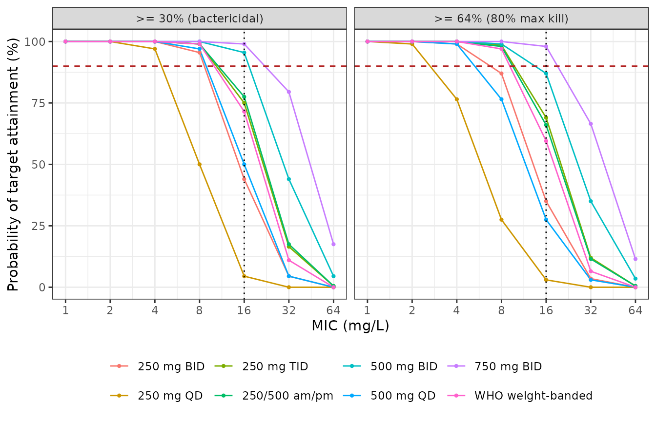
Simulated probability of target attainment against MIC for both hollow-fibre targets. Replicates Figure 3 of Resendiz-Galvan 2025.
The simulation reproduces the paper’s central conclusion: at the cohort median MIC of 16 mg/L only 500 mg BID and 750 mg BID reach high attainment of the preferred %T>MIC >= 64% target, while 250 mg QD is inadequate at any target.
Observed exposures reported in the source
For context, the paper’s observed (not simulated) intensive-sampling exposures, which the model was fit to.
| Regimen | Observed Cmax (mg/L) | Observed AUC0-24 (mg*h/L) |
|---|---|---|
| 250 mg BID | 16.8 (range 6.21-26.8) | 347.4 (IQR 261.1-425.7) |
| 250/500 am/pm | 30.5 (range 27.3-33.7) | 415.7 (IQR 224.1-553.9) |
Median tmax is computed here directly from the profile
over the first 12-hour interval of the steady-state day
in the 250 mg BID arm, i.e. time after a single observed morning dose –
which is what the paper’s intensive sampling (pre-dose, 1, 2, 4, 6, 8 h)
measured. (PKNCA’s interval-level tmax spans the whole 24 h
and can land on the evening peak, so it is not the right quantity
here.)
tmax_sim <- sim |>
  dplyr::filter(treatment == "250 mg BID", time <= t_ss + 12) |>
  dplyr::group_by(id) |>
  dplyr::slice_max(Cc, n = 1, with_ties = FALSE) |>
  dplyr::ungroup() |>
  dplyr::mutate(tmax = time - t_ss)

sprintf(
  "Simulated tmax after the morning dose: median %.2f h (IQR %.2f-%.2f); paper: 2 h (IQR 1.2-2.2)",
  median(tmax_sim$tmax), quantile(tmax_sim$tmax, 0.25), quantile(tmax_sim$tmax, 0.75)
)
#> [1] "Simulated tmax after the morning dose: median 2.40 h (IQR 1.68-3.40); paper: 2 h (IQR 1.2-2.2)"
stopifnot(median(tmax_sim$tmax) > 1, median(tmax_sim$tmax) < 4)
Assumptions and deviations
-
Allometric exponents are not printed in the source.
The paper states that allometric scaling on FFM was applied to the
disposition parameters and cites Holford for the renal/non-renal
separation, but Table 2 has no exponent row and the exponents appear
nowhere in the text or supplement, i.e. they were not estimated. They
are encoded as the standard theory-based values
(
fixed(0.75)on clearance,fixed(1)on volume). Every AUC in Table 3 is reproduced to within ~2% under this reading, which corroborates it. -
Table 1 mislabels the serum-creatinine unit as
mg/L. The printed Cockcroft-Gault equation reads
72 . SCr (mg/dL), and the arithmetic settles it: the median individual (age 27, SCr 0.7 mg/dL) gives CLcr,56M = 125.6 mL/min, consistent with the stated median of 122 mL/min, whereas mg/L would give ~1,256 mL/min. The model uses mg/dL. -
The clearance equation lost its parentheses in
typesetting. The text version reads
CL = CLnr + RF . CLr . Fsize, which would apply allometry to the renal arm only. The typeset equation image supplied with the article (aac.00101-25.m003) showsCL = (CLnr + RF . CLr) . Fsize, matching the prose (“the effect of body size Fsize … is applied to the overall CL (CLr + CLnr)”) and Table 2 footnote a (“All disposition parameters were allometrically scaled”). The parenthesised form is implemented. -
%CV convention. Table 2 footnote f defines %CV =
sqrt(omega^2) x 100, so the tabulated variability numbers are 100 x
omega on the log scale. Variances are therefore encoded as
(CV/100)^2, notlog((CV/100)^2 + 1). - The 250 mg BID row of Table 3 is inconsistent with the paper’s own model (see the dedicated section above). No parameter was tuned to match it.
-
Between-occasion variability is encoded over two occasion
types (
OCC = 1unobserved home dose,OCC = 2observed clinic dose), which is the distinction the 2.26-fold inflation factor is defined against. Whether that factor scales the BOV standard deviation or its variance is not stated; the SD reading is implemented, following the NONMEM idiom and the registry precedent inWojciechowski_2023_ritlecitinib_*.R. This vignette simulates fully-observed regimens (OCC = 2), where the factor is inactive and the ambiguity has no effect. -
useLinCmt = FALSEis mandatory for this model. It is a one-compartment oral model, so rxode2’s automatic ODE-to-linCmt()conversion fires. The converted form drops thetransit()input term, and because the model setsf(depot) <- 0(the dose enters only via the transit chain) the effective dose becomes zero and every concentration is zero – silently, with no error or warning. The simulation chunk assertsmax(Cc) > 1to make that failure mode loud. - Cohort covariate distributions are independent marginals. Weight, height, age, and serum creatinine are drawn at evenly-spaced quantiles of log-normals matched to their Table 1 medians and IQRs, then permuted independently; the paper reports no correlation structure between them. Stratifying rather than sampling at random is deliberate: the Table 1 marginals are a specification to reproduce, and at n = 200 random draws shift the cohort FFM median by ~3.6%, which alone biases every exposure by ~5%. The reproduced medians now match Table 1 to the reported precision. The derived FFM IQR is still modestly narrower than Table 1’s (34.3-45.4 vs 32.3-47.1 kg) because weight and height are independent here while in reality they correlate, so the simulated exposure spread is a little tighter than the published spread.
- A residual ~2-5% shortfall in simulated AUC remains across all regimens relative to Table 3. The paper’s virtual population was built from “repetitions of the original data set”, i.e. the real subjects’ joint covariate vectors, whereas this cohort samples the marginals independently. That is the most likely source; no parameter was adjusted to close the gap.
- Residual-error inflation for imputed records is not carried. The source inflated the additive error by LOD/2 for the three below-limit-of-detection records it imputed under an M6 adaptation (0.2% of observations). That record-specific adjustment is not representable as a model-level parameter and is omitted.
- Erratum. The article was published 2 September 2025 and reposted 1 October 2025 correcting the author-contributions statement only. No model parameter was revised; the version used is the corrected one. ```