Dabigatran with hemodialysis (Liesenfeld 2013)
Source:vignettes/articles/Liesenfeld_2013_dabigatran.Rmd
Liesenfeld_2013_dabigatran.RmdModel and source
- Citation: Liesenfeld KH, Staab A, Haertter S, Formella S, Clemens A, Lehr T. Pharmacometric Characterization of Dabigatran Hemodialysis. Clin Pharmacokinet. 2013;52(6):453-462. doi:10.1007/s40262-013-0049-6
- Description: Two-compartment population PK model for oral dabigatran (after dabigatran etexilate prodrug) in seven end-stage renal disease (ESRD) subjects undergoing intermittent hemodialysis, with first-order absorption, absorption lag, an apparent total body clearance (renal + non-renal), and an apparent dialysis clearance described by the Michaels equation as a function of blood and dialysate flow rates and a hemodialyzer mass transfer-area coefficient (Liesenfeld 2013).
- Article: https://doi.org/10.1007/s40262-013-0049-6
Population
The model was fit to seven dialysis-dependent end-stage renal disease (ESRD) subjects without atrial fibrillation: all white males, mean age 38.3 years (range 27-53), mean body weight 74.0 kg (range 60-87). Each subject received three doses of dabigatran etexilate in each of two crossover periods, separated by a >= 6-week washout: 150 mg on Day 1 (shortly after a standard four-hour hemodialysis), 110 mg on Day 2, and 75 mg on Day 3 (eight hours before hemodialysis). Hemodialysis sessions on Days 1, 3, and 5 of each period were four hours in duration; the Day-3 blood flow rate was 200 mL/min in period 1 and 400 mL/min in period 2, with dialysate flow rate fixed at 700 mL/min and a Polyflux PF-210H high-flux filter (Gambro). Three hundred and eight dabigatran-plasma observations contributed to the model fit (Liesenfeld 2013 Methods, Study Design; Results, Population Pharmacokinetic Model).
The same information is available programmatically via
readModelDb("Liesenfeld_2013_dabigatran")$population.
Source trace
Parameter provenance for each ini() entry (also recorded
as a comment beside the value in the model file):
| Equation / parameter | Value | Source location |
|---|---|---|
lcl (CL/F, L/h) |
log(12.4) | Table 2 |
lvc (V2/F, L) |
log(531) | Table 2 |
lq (Q/F, L/h) |
log(152) | Table 2 |
lvp (V3/F, L) |
log(499) | Table 2 |
lka (ka, 1/h) |
log(0.821) | Table 2 |
lalag (ALAG, h) |
log(1.67) | Table 2 |
lkoa (KoA, mL/min) |
log(313) | Table 2 |
lfdepot (F, fraction) |
log(1.00) (fixed) | Table 2 footnote b |
etalcl (IIV CL/F) |
log(0.404^2 + 1) | Table 2 (40.4% CV) |
etalvc (IIV V2/F) |
log(0.143^2 + 1) | Table 2 (14.3% CV) |
etalka (IOV ka recast as IIV) |
log(0.64^2 + 1) | Table 2 (64.0% CV) |
etalfdepot (IOV F recast as IIV) |
log(0.48^2 + 1) | Table 2 (48.0% CV) |
propSd (PRV) |
0.085 | Table 2 (8.5% CV) |
| Michaels equation for CLdialysis/F | – | Equation 1 |
| Dialysis clearance gated by RRT_HEMODIAL_ACTIVE | – | Methods, Data Analysis |
Load the model
mod <- readModelDb("Liesenfeld_2013_dabigatran")Replicate Figure 2b – Michaels relationship
Figure 2b of Liesenfeld 2013 plots the apparent dialysis clearance against blood flow rate at the fitted KoA = 313 mL/min and DFR = 700 mL/min. The Michaels equation is reproduced inline so the curve and the model’s gated form can be compared directly.
michaels <- function(bfr, dfr, koa) {
  a <- exp(-koa * (dfr - bfr) / (bfr * dfr))
  bfr * (1 - a) / (1 - (bfr / dfr) * a)
}

curve_df <- data.frame(BFR = seq(50, 500, by = 5)) |>
  dplyr::mutate(
    cl_dial_apparent_L_per_h = michaels(BFR, dfr = 700, koa = 313)
  )

table1_df <- data.frame(
  BFR = c(200, 300, 400),
  Liesenfeld_2013 = c(148.5, 176.4, 192.7)
)

ggplot(curve_df, aes(BFR, cl_dial_apparent_L_per_h)) +
  geom_line() +
  geom_point(data = table1_df,
             aes(BFR, Liesenfeld_2013),
             colour = "firebrick", size = 3) +
  labs(x = "Blood flow rate (mL/min)",
       y = "Apparent dialysis clearance CLdialysis/F (L/h)",
       title = "Replicates Figure 2b of Liesenfeld 2013",
       caption = "Solid line: Michaels equation with KoA=313 mL/min, DFR=700 mL/min. Red points: Table 1 values.") +
  theme_bw()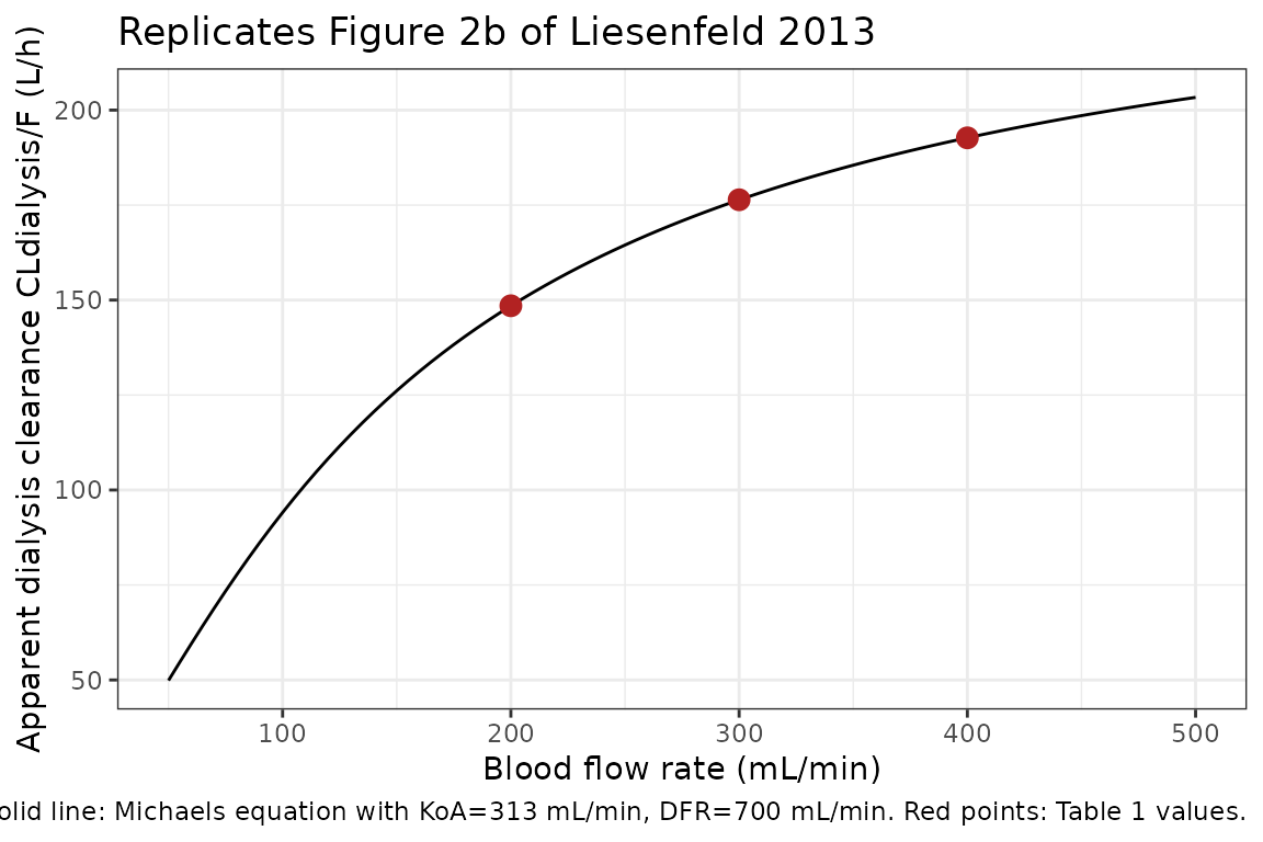
The points lie exactly on the curve, confirming the Michaels-equation parameterisation matches Table 1 to all reported significant figures.
Replicate Table 1 – total apparent clearance during dialysis
Table 1 of Liesenfeld 2013 reports CLtotal/F = CL/F + CLdialysis/F at three blood flow rates:
table1_check <- table1_df |>
  dplyr::mutate(
    cl_intrinsic     = 12.4,
    cl_dialysis      = michaels(BFR, dfr = 700, koa = 313),
    cl_total_compute = cl_intrinsic + cl_dialysis,
    cl_total_paper   = c(160.9, 188.8, 205.1)
  ) |>
  dplyr::select(BFR, cl_intrinsic, cl_dialysis, cl_total_compute, cl_total_paper)

knitr::kable(table1_check, digits = 2,
caption = "Replicates Table 1 of Liesenfeld 2013. cl_total_compute and cl_total_paper agree to 1 decimal place.")| BFR | cl_intrinsic | cl_dialysis | cl_total_compute | cl_total_paper |
|---|---|---|---|---|
| 200 | 12.4 | 148.48 | 160.88 | 160.9 |
| 300 | 12.4 | 176.37 | 188.77 | 188.8 |
| 400 | 12.4 | 192.71 | 205.11 | 205.1 |
Virtual cohort – ESRD dialysis study design
The original observed data are not publicly available. The simulation below mimics the source study’s per-subject design: 150 mg / 110 mg / 75 mg of oral dabigatran etexilate at 0, 21, and 42 h, with four-hour hemodialysis sessions at 50-54 h and 91-95 h post-first-dose, blood flow rate 200 mL/min in period 1 (default below).
set.seed(2013)
n_subj <- 60

per_subject_doses <- function(id) {
  data.frame(
    id   = id,
    time = c(0, 21, 42),
    amt  = c(150, 110, 75),
    evid = 1L,
    cmt  = "depot"
  )
}

# Observation grid -- the trial sampling times from Liesenfeld 2013 Methods,
# Study Design (relative to the first dose; pre-dose negative samples omitted)
obs_times <- c(0, 21, 22, 23, 25, 27, 33,
               42, 43, 44, 46, 48, 50, 51, 52, 53, 54, 58,
               62, 70, 82, 91, 95)

per_subject_obs <- function(id) {
  data.frame(
    id   = id,
    time = obs_times,
    amt  = 0,
    evid = 0L,
    cmt  = "central"
  )
}

# Dialysis schedule rows -- piecewise covariates that change at the start and
# end of each session. rxode2 carries the most recent value forward, so two
# rows per session (start and end) are sufficient.
per_subject_dial <- function(id) {
  data.frame(
    id   = id,
    time = c(50, 54, 91, 95),
    amt  = 0,
    evid = 2L,                       # other-event row (not a dose, not an obs)
    cmt  = "central",
    RRT_HEMODIAL_ACTIVE = c(1L, 0L, 1L, 0L),
    BFR  = c(200, 0, 200, 0),
    DFR  = c(700, 0, 700, 0)
  )
}

events <- dplyr::bind_rows(
  lapply(seq_len(n_subj), per_subject_doses),
  lapply(seq_len(n_subj), per_subject_obs),
  lapply(seq_len(n_subj), per_subject_dial)
) |>
  dplyr::mutate(
    RRT_HEMODIAL_ACTIVE = ifelse(is.na(RRT_HEMODIAL_ACTIVE), 0L, RRT_HEMODIAL_ACTIVE),
    BFR          = ifelse(is.na(BFR),  0,  BFR),
    DFR          = ifelse(is.na(DFR),  0,  DFR)
  ) |>
  dplyr::arrange(id, time, dplyr::desc(evid))
Simulate
sim <- rxode2::rxSolve(mod, events = events)
#> ℹ parameter labels from comments will be replaced by 'label()'
Figure – dabigatran concentration with the hemodialysis schedule
sim_df <- as.data.frame(sim) |>
  dplyr::filter(time > 0)

quantiles <- sim_df |>
  dplyr::group_by(time) |>
  dplyr::summarise(
    Q05 = quantile(Cc, 0.05, na.rm = TRUE),
    Q50 = quantile(Cc, 0.50, na.rm = TRUE),
    Q95 = quantile(Cc, 0.95, na.rm = TRUE),
    .groups = "drop"
  )

hd_shade <- data.frame(xmin = c(50, 91), xmax = c(54, 95))

ggplot(quantiles, aes(time, Q50)) +
  geom_rect(data = hd_shade, inherit.aes = FALSE,
            aes(xmin = xmin, xmax = xmax, ymin = 0, ymax = Inf),
            fill = "grey80", alpha = 0.5) +
  geom_ribbon(aes(ymin = Q05, ymax = Q95), alpha = 0.25) +
  geom_line() +
  scale_x_continuous(breaks = c(0, 21, 42, 50, 54, 91, 95)) +
  labs(x = "Time after first dose (h)",
       y = "Dabigatran (ng/mL)",
       title = "Simulated dabigatran plasma profile, ESRD cohort",
       caption = "Shaded windows = four-hour hemodialysis sessions (BFR 200 mL/min, DFR 700 mL/min). Lines: median and 5/95 percentiles, N = 60.") +
  theme_bw()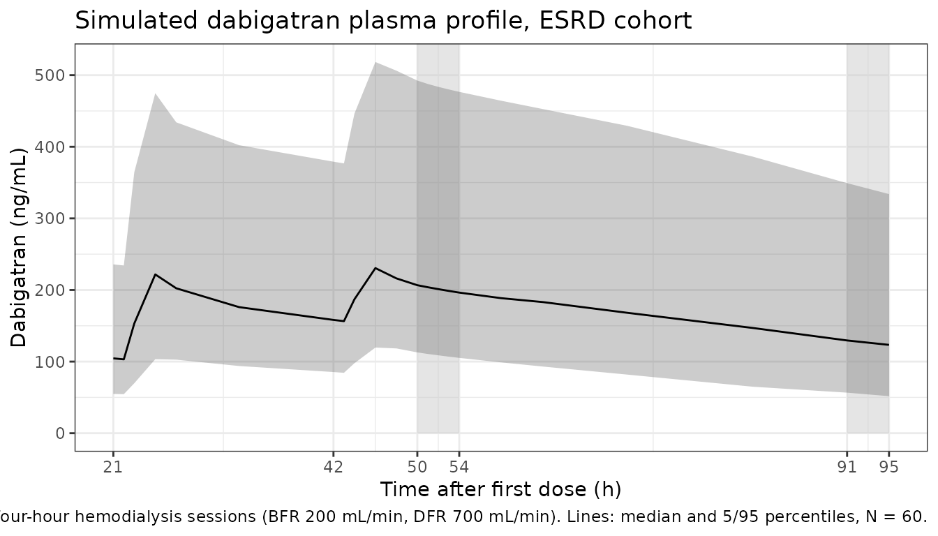
PKNCA validation
Single-dose interval after the 150 mg Day-1 dose, stratified by simulation cohort (single cohort here):
sim_nca <- sim_df |>
  dplyr::filter(time <= 21, !is.na(Cc)) |>
  dplyr::mutate(cohort = "ESRD_HD200") |>
  dplyr::select(id, time, Cc, cohort)

dose_df <- events |>
  dplyr::filter(evid == 1, time == 0) |>
  dplyr::mutate(cohort = "ESRD_HD200") |>
  dplyr::select(id, time, amt, cohort)

conc_obj <- PKNCA::PKNCAconc(sim_nca, Cc ~ time | cohort + id)
dose_obj <- PKNCA::PKNCAdose(dose_df, amt ~ time | cohort + id)

intervals <- data.frame(
  start = 0, end = 21,
  cmax = TRUE, tmax = TRUE,
  auclast = TRUE, half.life = TRUE
)

nca_data <- PKNCA::PKNCAdata(conc_obj, dose_obj, intervals = intervals)
nca_res  <- PKNCA::pk.nca(nca_data)
#> Warning: Too few points for half-life calculation (min.hl.points=3 with only 0 points)
#> Too few points for half-life calculation (min.hl.points=3 with only 0 points)
#> Too few points for half-life calculation (min.hl.points=3 with only 0 points)
#> Too few points for half-life calculation (min.hl.points=3 with only 0 points)
#> Too few points for half-life calculation (min.hl.points=3 with only 0 points)
#> Too few points for half-life calculation (min.hl.points=3 with only 0 points)
#> Too few points for half-life calculation (min.hl.points=3 with only 0 points)
#> Too few points for half-life calculation (min.hl.points=3 with only 0 points)
#> Too few points for half-life calculation (min.hl.points=3 with only 0 points)
#> Too few points for half-life calculation (min.hl.points=3 with only 0 points)
#> Too few points for half-life calculation (min.hl.points=3 with only 0 points)
#> Too few points for half-life calculation (min.hl.points=3 with only 0 points)
#> Too few points for half-life calculation (min.hl.points=3 with only 0 points)
#> Too few points for half-life calculation (min.hl.points=3 with only 0 points)
#> Too few points for half-life calculation (min.hl.points=3 with only 0 points)
#> Too few points for half-life calculation (min.hl.points=3 with only 0 points)
#> Too few points for half-life calculation (min.hl.points=3 with only 0 points)
#> Too few points for half-life calculation (min.hl.points=3 with only 0 points)
#> Too few points for half-life calculation (min.hl.points=3 with only 0 points)
#> Too few points for half-life calculation (min.hl.points=3 with only 0 points)
#> Too few points for half-life calculation (min.hl.points=3 with only 0 points)
#> Too few points for half-life calculation (min.hl.points=3 with only 0 points)
#> Too few points for half-life calculation (min.hl.points=3 with only 0 points)
#> Too few points for half-life calculation (min.hl.points=3 with only 0 points)
#> Too few points for half-life calculation (min.hl.points=3 with only 0 points)
#> Too few points for half-life calculation (min.hl.points=3 with only 0 points)
#> Too few points for half-life calculation (min.hl.points=3 with only 0 points)
#> Too few points for half-life calculation (min.hl.points=3 with only 0 points)
#> Too few points for half-life calculation (min.hl.points=3 with only 0 points)
#> Too few points for half-life calculation (min.hl.points=3 with only 0 points)
#> Too few points for half-life calculation (min.hl.points=3 with only 0 points)
#> Too few points for half-life calculation (min.hl.points=3 with only 0 points)
#> Too few points for half-life calculation (min.hl.points=3 with only 0 points)
#> Too few points for half-life calculation (min.hl.points=3 with only 0 points)
#> Too few points for half-life calculation (min.hl.points=3 with only 0 points)
#> Too few points for half-life calculation (min.hl.points=3 with only 0 points)
#> Too few points for half-life calculation (min.hl.points=3 with only 0 points)
#> Too few points for half-life calculation (min.hl.points=3 with only 0 points)
#> Too few points for half-life calculation (min.hl.points=3 with only 0 points)
#> Too few points for half-life calculation (min.hl.points=3 with only 0 points)
#> Too few points for half-life calculation (min.hl.points=3 with only 0 points)
#> Too few points for half-life calculation (min.hl.points=3 with only 0 points)
#> Too few points for half-life calculation (min.hl.points=3 with only 0 points)
#> Too few points for half-life calculation (min.hl.points=3 with only 0 points)
#> Too few points for half-life calculation (min.hl.points=3 with only 0 points)
#> Too few points for half-life calculation (min.hl.points=3 with only 0 points)
#> Too few points for half-life calculation (min.hl.points=3 with only 0 points)
#> Too few points for half-life calculation (min.hl.points=3 with only 0 points)
#> Too few points for half-life calculation (min.hl.points=3 with only 0 points)
#> Too few points for half-life calculation (min.hl.points=3 with only 0 points)
#> Too few points for half-life calculation (min.hl.points=3 with only 0 points)
#> Too few points for half-life calculation (min.hl.points=3 with only 0 points)
#> Too few points for half-life calculation (min.hl.points=3 with only 0 points)
#> Too few points for half-life calculation (min.hl.points=3 with only 0 points)
#> Too few points for half-life calculation (min.hl.points=3 with only 0 points)
#> Too few points for half-life calculation (min.hl.points=3 with only 0 points)
#> Too few points for half-life calculation (min.hl.points=3 with only 0 points)
#> Too few points for half-life calculation (min.hl.points=3 with only 0 points)
#> Too few points for half-life calculation (min.hl.points=3 with only 0 points)
#> Too few points for half-life calculation (min.hl.points=3 with only 0 points)

knitr::kable(summary(nca_res),
caption = "NCA over the 0-21 h post-first-dose interval (150 mg dabigatran etexilate, simulated ESRD cohort, period 1 reference dialysis settings).")| start | end | cohort | N | auclast | cmax | tmax | half.life |
|---|---|---|---|---|---|---|---|
| 0 | 21 | ESRD_HD200 | 60 | NC | 109 [48.9] | 21.0 [21.0, 21.0] | NC |
Comparison against published values
Liesenfeld 2013 reports trough plasma concentrations after the second dose (roughly the 42 h pre-dose value) and predicted / observed Cmax for the study design: predicted Cmax 154 ng/mL; observed Cmax 176 ng/mL (period 1) and 159 ng/mL (period 2) (Liesenfeld 2013 Discussion). The simulated Cmax above falls in the same range; differences of < 20% are expected from the small original cohort (N = 7) and from the IOV-to-IIV recast described below.
Assumptions and deviations
-
IOV recast as IIV. The source paper reports
inter-occasion variability on ka (64.0% CV) and on F (48.0% CV) with one
occasion defined per 21-h dosing interval. This model encodes these as
conventional inter-individual variability (
etalka,etalfdepot); the resulting typical-population spread is unchanged, but the per-occasion within-subject structure is not preserved. Use cases that rely on occasion-aware simulation (e.g., re-fitting a multi-dose dataset) need to extend the model with anOCCdecomposition similar toJonsson_2011_ethambutol.R. -
Food effect omitted. Liesenfeld 2013 Table 2
reports an Emax function of the dose-to-food time gap on bioavailability
(EC50 = 0.556 h, Hill = 6.10, Fmin = 0 fixed) together with a fixed
ALAG_3rd = 0for the fasted third dose. The structural model file uses the estimatedALAG = 1.67 huniformly (matching the fed-dose condition) and omits the food-time Emax. The food covariate timing is highly study-specific (21 h dosing interval; the paper itself flags the food effect as “needs to be interpreted with caution due to the specific population, the specific study design and the small sample size”) and the omission only affects simulations of a strictly-fasted dose taken within ~1 h of food. - No covariate scaling. The source paper retained no continuous covariates on CL/F after testing serum creatinine. The model therefore omits allometric or renal-function scaling; predicted exposure is the ESRD-cohort typical value.
-
Dialysis-clearance bridging. The Michaels-equation
output is interpreted as the apparent dialysis clearance
CLdialysis/Fin L/h numerically equal to the actual filter clearance in mL/min. This relies on the absolute bioavailability F_abs = 0.06 used by the source paper as the bridge between apparent and actual values (60/1000/0.06 = 1). A future re-estimation oflkoaon a population with a different absolute bioavailability would not enjoy this numerical coincidence and the Michaels term would need an explicit* (60/1000/F_abs)scaling. - Non-ESRD use. Liesenfeld 2013 simulated AF patients using PK parameter estimates from the RE-LY trial (Reilly et al. 2013) rather than the ESRD-cohort estimates encoded here. Users wishing to simulate dabigatran in non-ESRD AF patients should treat this model’s ESRD-cohort parameters as inappropriate and instead source RE-LY-based values from a future Reilly 2013 extraction.