Vinpocetine / apovincaminic acid (Petric 2023)
Source:vignettes/articles/Petric_2023_vinpocetine.Rmd
Petric_2023_vinpocetine.Rmd
library(nlmixr2lib)
library(PKNCA)
#>
#> Attaching package: 'PKNCA'
#> The following object is masked from 'package:stats':
#>
#>     filter
library(rxode2)
#> rxode2 5.1.8 using 2 threads (see ?getRxThreads)
#>   no cache: create with `rxCreateCache()`
library(dplyr)
#>
#> Attaching package: 'dplyr'
#> The following objects are masked from 'package:stats':
#>
#>     filter, lag
#> The following objects are masked from 'package:base':
#>
#>     intersect, setdiff, setequal, union
library(tidyr)
library(ggplot2)
Model and source
- Citation: Petric Z, Paixao P, Filipe A, Guimaraes Morais J. Clinical Pharmacology of Vinpocetine: Properties Revisited and Introduction of a Population Pharmacokinetic Model for Its Metabolite, Apovincaminic Acid (AVA). Pharmaceutics. 2023;15(10):2502.
- DOI: https://doi.org/10.3390/pharmaceutics15102502
- Article (open access): https://www.mdpi.com/1999-4923/15/10/2502
The paper is open access under CC BY 4.0. A brief supplement (Table S1 demographics, Table S2 OFV / AIC / BIC comparison) is available from the same publisher page.
Population
Petric 2023 fits a two-compartment population PK model of the active vinpocetine metabolite apovincaminic acid (AVA) to plasma AVA concentrations from 12 healthy adult male volunteers (Portugal) enrolled in an open crossover relative-bioavailability study. Each subject received all three formulations of vinpocetine (a single 20 mg oral dose per occasion) with a 7-day washout between formulations:
- Formulation #1 – Ultra Vinca (Tecnimede, Portugal): sustained-release beta-cyclodextrin-complex 10 mg tablets (2 tablets = 20 mg per occasion). This is the reference formulation for the covariate parameterisation (Petric 2023 Table 1).
- Formulation #2 – Cavinton (Organon / Gedeon Richter, Hungary): immediate-release 5 mg tablets (4 tablets = 20 mg per occasion).
- Formulation #3 – extemporaneous oral solution prepared at the hospital pharmacy from the pure API supplied by Tecnimede (5 mL / 10 mg concentration, 10 mL = 20 mg per occasion).
Plasma AVA was sampled between 0.25 h and 10 h post-dose and quantified by HPLC-UV at 254 nm (linear range 5-300 ng/mL, LLOQ 5 ng/mL, R.S.D. ~7 %). BLQ observations were retained (not censored) per Petric 2023 Section 3.3.
Baseline demographics (Petric 2023 Supplementary Table S1):
| Covariate | Min | Median | Max |
|---|---|---|---|
| Age (years) | 20 | 23 | 35 |
| BMI (kg/m^2) | 20.9 | 24.9 | 32.56 |
| Height (m) | 1.64 | 1.74 | 1.83 |
| Weight (kg) | 66 | 73.5 | 93 |
All subjects were male. Age, height, weight (as BMI), and formulation
were screened as candidate covariates using a stepwise procedure; only
formulation was retained (on Tk0 and V1/F). The full
population metadata is available programmatically via
readModelDb("Petric_2023_vinpocetine")()$population.
Source trace
Every value below is tagged in-line in
inst/modeldb/specificDrugs/Petric_2023_vinpocetine.R. This
table collects the provenance in one place.
| Equation / parameter | Value | Source location |
|---|---|---|
Tlag_pop (exp(ltlag)) |
0.17 h | Table 1, “Tlag_pop” |
Tk0_pop (exp(ld1) at Formulation#1) |
1.35 h | Table 1, “Tk0_pop” |
beta_Tk0_Formulation#2
(e_form_ir_ld1) |
-0.4 | Table 1, “beta_Tk0_Formulation#2” |
beta_Tk0_Formulation#3
(e_form_sol_ld1) |
-0.68 | Table 1, “beta_Tk0_Formulation#3” |
CL/F_pop (exp(lcl)) |
56.15 L/h | Table 1, “Cl/F_pop L/h” |
V1/F_pop (exp(lvc) at Formulation#1) |
208.34 L | Table 1, “V1/F_pop L” |
beta_V1/F_Formulation#2
(e_form_ir_lvc) |
-1.26 | Table 1, “beta_V1/F_Formulation#2” |
beta_V1/F_Formulation#3
(e_form_sol_lvc) |
-1.24 | Table 1, “beta_V1/F_Formulation#3” |
Q/F_pop (exp(lq)) |
14.63 L/h | Table 1, “Q/F_pop L” (unit typo – see Errata) |
V2/F_pop (exp(lvp)) |
76.15 L | Table 1, “V2/F_pop L” |
omega_Tlag (sqrt(var(etaltlag))) |
0.38 | Table 1, “omega_Tlag” |
omega_Tk0 (sqrt(var(etald1))) |
0.24 | Table 1, “omega_Tk0” |
omega_Cl/F |
0.21 | Table 1, “omega_Cl/F” |
omega_V1/F |
0.15 | Table 1, “omega_V1/F” |
corr_V1/F_Cl/F |
0.72 | Table 1, “Correlations: corr_V1/F_Cl/F” |
omega_Q/F |
0.47 | Table 1, “omega_Q/F” |
omega_V2/F |
0.24 | Table 1, “omega_V2/F” |
Residual error (proportional b) |
0.14 | Table 1, “b” |
d/dt(central) = -kel * central - k12 * central + k21 * peripheral1 |
n/a | Section 3.3 “two-compartment … zero-order input”; Table 1 abbreviations |
dur(central) <- Tk0,
alag(central) <- Tlag
|
n/a | Section 3.3 “zero-order input … lag time before absorption” |
Cc scaling central / vc * 1000
|
mg -> ug/L | Table 1 unit key (“V1/F_pop L”, concentration reported in ug/L per Fig 2/4/5) |
Virtual cohort
The Petric 2023 study is a within-subject 3-formulation crossover in
12 healthy adult male volunteers. This vignette replicates the study
design directly: 12 virtual subjects, each carried across all three
formulations with a distinct integer id per (subject,
formulation) combination so rxSolve does not collapse them
(subject-plus-formulation combos become 12 x 3 = 36 disjoint IDs – well
below the 200/arm cap).
The FORM_VINP_IR and FORM_SOLUTION indicator pair encodes the three-level categorical formulation covariate. Formulation #1 (Ultra Vinca SR beta-cyclodextrin) is the reference (both indicators = 0). No continuous covariate is used in the final model, so the demographic distributions reported in Supplementary Table S1 do not enter the simulation.
set.seed(20231020)

n_subj <- 12L

formulations <- tibble::tribble(
  ~formulation,        ~FORM_VINP_IR, ~FORM_SOLUTION, ~formulation_short,
  "SR beta-cyclodextrin", 0L,          0L,             "SR (Ultra Vinca)",
  "IR tablet",            1L,          0L,             "IR (Cavinton)",
  "Oral solution",        0L,          1L,             "Solution"
)

# One row per subject-formulation combination. IDs are disjoint across
# formulations so rxSolve treats them as separate simulated subjects.
cohort <- tidyr::expand_grid(
  subject     = seq_len(n_subj),
  formulation = formulations$formulation
) |>
  dplyr::left_join(formulations, by = "formulation") |>
  dplyr::mutate(id = seq_len(dplyr::n()))

# Dose records: single 20 mg vinpocetine dose into the central compartment as
# a zero-order input. The `dur(central) <- d1` in the model file supplies the
# duration from the individual d1 parameter, so we set `rate = -2` on the dose
# to select model-supplied duration semantics.
dose_recs <- cohort |>
  dplyr::mutate(
    time = 0,
    amt  = 20,
    evid = 1L,
    cmt  = "central",
    rate = -2
  )

# Observation records: 0.25 h to 10 h, matching the paper's sampling window
# (Section 2.2). Additional pre-dose t = 0 row is added later for NCA anchoring.
obs_times <- c(0, 0.25, 0.5, 0.75, 1, 1.5, 2, 2.5, 3, 4, 5, 6, 7, 8, 9, 10)
obs_recs <- cohort |>
  tidyr::expand_grid(time = obs_times) |>
  dplyr::mutate(
    amt  = 0,
    evid = 0L,
    cmt  = "central",
    rate = 0
  )

events <- dplyr::bind_rows(dose_recs, obs_recs) |>
  dplyr::arrange(id, time, dplyr::desc(evid)) |>
  dplyr::select(id, time, amt, evid, cmt, rate,
                formulation, formulation_short,
                FORM_VINP_IR, FORM_SOLUTION)

stopifnot(!anyDuplicated(unique(events[, c("id", "time", "evid")])))
Simulation
Two simulations are performed:
-
Typical-value simulation
(
rxode2::zeroRe()) – the deterministic population profile, used to reproduce the paper’s Figure 2 and to seed the PKNCA validation table. - Stochastic VPC – full between-subject variability from the packaged omegas, used to reproduce Figure 4A/B.
mod <- readModelDb("Petric_2023_vinpocetine")

sim_typical <- rxode2::rxSolve(
  rxode2::zeroRe(mod),
  events = events,
  keep   = c("formulation", "formulation_short")
) |>
  as.data.frame()
#> ℹ parameter labels from comments will be replaced by 'label()'
#> ℹ omega/sigma items treated as zero: 'etaltlag', 'etald1', 'etalcl', 'etalvc', 'etalq', 'etalvp'
#> Warning: multi-subject simulation without without 'omega'

# Stochastic VPC -- replicate the 12-subject crossover 50 times per formulation
# (600 virtual subjects per formulation arm; 3 * 200 = 600 <= 200/arm applied to
# the *per-formulation* population). Random effects are drawn from the packaged
# variance-covariance matrix.
n_vpc_replicates <- 200L / n_subj  # -> 16 replicates x 12 subjects = 192/arm
vpc_cohort <- tidyr::expand_grid(
  replicate   = seq_len(n_vpc_replicates),
  subject     = seq_len(n_subj),
  formulation = formulations$formulation
) |>
  dplyr::left_join(formulations, by = "formulation") |>
  dplyr::mutate(id = seq_len(dplyr::n()))

vpc_dose <- vpc_cohort |>
  dplyr::mutate(time = 0, amt = 20, evid = 1L, cmt = "central", rate = -2)
vpc_obs <- vpc_cohort |>
  tidyr::expand_grid(time = seq(0, 10, by = 0.25)) |>
  dplyr::mutate(amt = 0, evid = 0L, cmt = "central", rate = 0)
vpc_events <- dplyr::bind_rows(vpc_dose, vpc_obs) |>
  dplyr::arrange(id, time, dplyr::desc(evid)) |>
  dplyr::select(id, time, amt, evid, cmt, rate,
                formulation, formulation_short, FORM_VINP_IR, FORM_SOLUTION)

sim_vpc <- rxode2::rxSolve(
  mod,
  events = vpc_events,
  keep   = c("formulation", "formulation_short")
) |>
  as.data.frame()
#> ℹ parameter labels from comments will be replaced by 'label()'
Replicate Figure 2 – mean plasma AVA by formulation
Petric 2023 Figure 2 shows the mean +/- SD plasma AVA vs. time curves for the three formulations at 20 mg vinpocetine, on a log-linear scale. The typical-value simulation reproduces the mean trend; the VPC simulation reproduces the between-subject variability (SD envelope).
sim_typical |>
  dplyr::filter(time > 0) |>
  ggplot(aes(time, Cc, colour = formulation_short)) +
  geom_line(linewidth = 0.9) +
  scale_y_log10() +
  labs(
    x       = "Time after 20 mg vinpocetine dose (h)",
    y       = "AVA concentration (ug/L, log10 scale)",
    colour  = "Formulation",
    title   = "Typical-value AVA plasma profiles by formulation",
    caption = "Replicates Petric 2023 Figure 2 (mean profiles). Formulation #1 (SR Ultra Vinca) is the model reference."
  ) +
  theme_bw()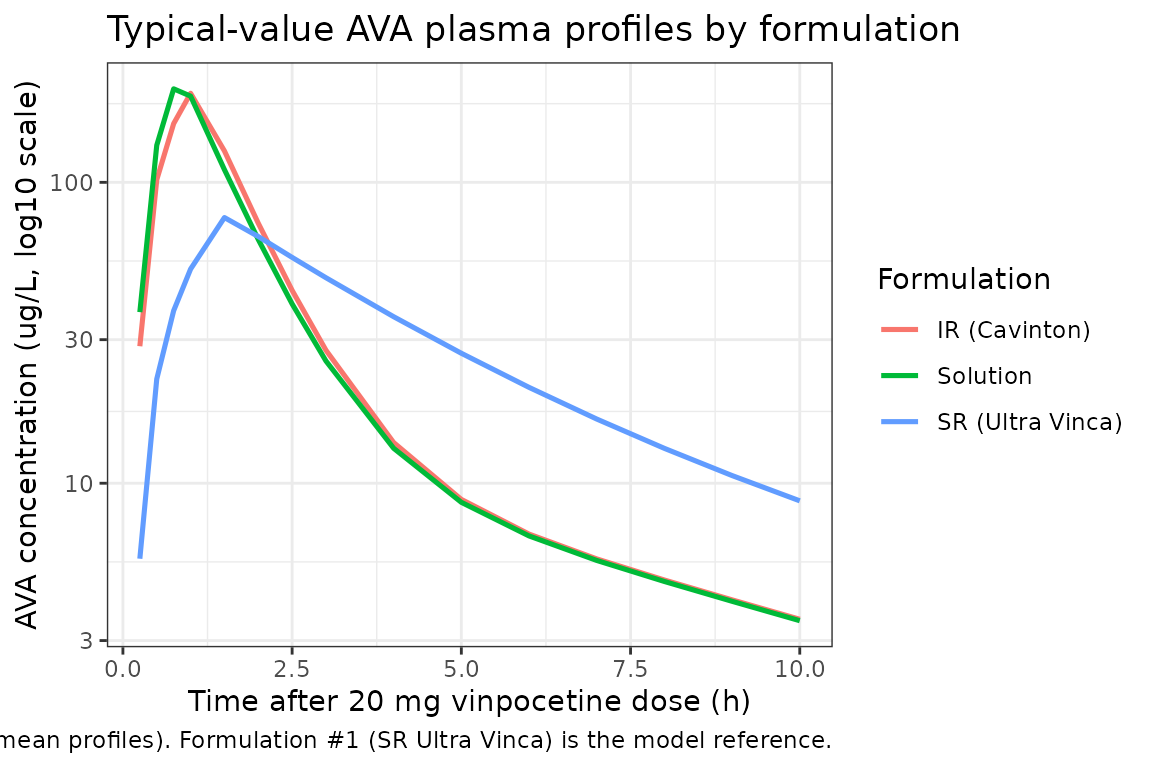
Replicate Figure 4 – stratified VPC by formulation
sim_vpc |>
  dplyr::filter(time > 0) |>
  dplyr::group_by(formulation_short, time) |>
  dplyr::summarise(
    Q10 = quantile(Cc, 0.10, na.rm = TRUE),
    Q50 = quantile(Cc, 0.50, na.rm = TRUE),
    Q90 = quantile(Cc, 0.90, na.rm = TRUE),
    .groups = "drop"
  ) |>
  ggplot(aes(time, Q50)) +
  geom_ribbon(aes(ymin = Q10, ymax = Q90), fill = "steelblue", alpha = 0.25) +
  geom_line(linewidth = 0.8, colour = "steelblue") +
  facet_wrap(~ formulation_short) +
  scale_y_log10() +
  labs(
    x       = "Time after 20 mg vinpocetine dose (h)",
    y       = "AVA concentration (ug/L, log10 scale)",
    title   = "Stratified VPC of AVA plasma profiles by formulation",
    caption = "Replicates Petric 2023 Figure 4B. Ribbon = 10th-90th percentile prediction interval; line = median."
  ) +
  theme_bw()
#> Warning in scale_y_log10(): log-10 transformation introduced infinite values.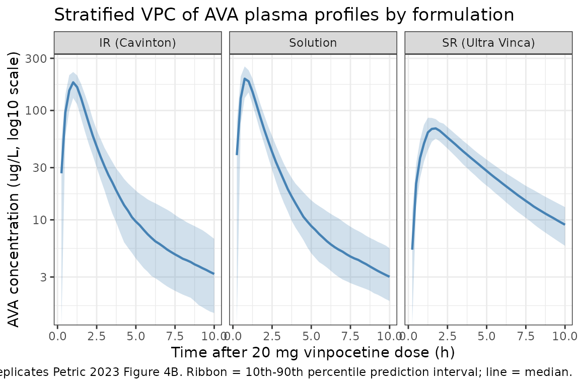
Simulated dose regimens – Figure 5 replication (partial)
Petric 2023 Figure 5c/d compare Cmax and Cmin distributions across six simulated multi-dose regimens of vinpocetine tablets. The two headline numbers reported in Section 3.5 for the Cavinton IR tablet (Formulation #2) are:
- 5 mg every 8 h, mean Cmax = 48.7 ug/L; mean Cmin = 1.25 ug/L
- 15 mg every 24 h, mean Cmax = 140.7 ug/L; mean Cmin = 0.52 ug/L
The two regimens below simulate 50 virtual individuals through 7 days of dosing so the Cmax and Cmin can be summarised on the last dosing interval.
# Simulate 50 virtual individuals on Formulation #2 (Cavinton IR) for each
# of the two headline regimens over 7 days of dosing. Total per-arm cohort
# = 50 <= 200/arm.
n_virt <- 50L

# Regimen 1: 5 mg every 8 h for 7 days -> 21 doses
r1_ids <- seq_len(n_virt)
r1_dose <- tidyr::expand_grid(id = r1_ids, time = (0:20) * 8) |>
  dplyr::mutate(amt = 5, evid = 1L, cmt = "central", rate = -2,
                FORM_VINP_IR = 1L, FORM_SOLUTION = 0L,
                regimen = "5 mg every 8 h")
r1_obs <- tidyr::expand_grid(id = r1_ids, time = seq(160, 168, by = 0.1)) |>
  dplyr::mutate(amt = 0, evid = 0L, cmt = "central", rate = 0,
                FORM_VINP_IR = 1L, FORM_SOLUTION = 0L,
                regimen = "5 mg every 8 h")

# Regimen 2: 15 mg every 24 h for 7 days -> 7 doses
r2_ids <- n_virt + seq_len(n_virt)
r2_dose <- tidyr::expand_grid(id = r2_ids, time = (0:6) * 24) |>
  dplyr::mutate(amt = 15, evid = 1L, cmt = "central", rate = -2,
                FORM_VINP_IR = 1L, FORM_SOLUTION = 0L,
                regimen = "15 mg every 24 h")
r2_obs <- tidyr::expand_grid(id = r2_ids, time = seq(144, 168, by = 0.1)) |>
  dplyr::mutate(amt = 0, evid = 0L, cmt = "central", rate = 0,
                FORM_VINP_IR = 1L, FORM_SOLUTION = 0L,
                regimen = "15 mg every 24 h")

fig5_events <- dplyr::bind_rows(r1_dose, r1_obs, r2_dose, r2_obs) |>
  dplyr::arrange(id, time, dplyr::desc(evid)) |>
  dplyr::select(id, time, amt, evid, cmt, rate, regimen,
                FORM_VINP_IR, FORM_SOLUTION)

stopifnot(!anyDuplicated(unique(fig5_events[, c("id", "time", "evid")])))

sim_fig5 <- rxode2::rxSolve(mod, events = fig5_events, keep = c("regimen")) |>
  as.data.frame()

# Cmax/Cmin over the LAST dosing interval per subject.
last_intervals <- dplyr::bind_rows(
  sim_fig5 |> dplyr::filter(regimen == "5 mg every 8 h",
                            time >= 160, time <= 168),
  sim_fig5 |> dplyr::filter(regimen == "15 mg every 24 h",
                            time >= 144, time <= 168)
)

fig5_summary <- last_intervals |>
  dplyr::group_by(id, regimen) |>
  dplyr::summarise(Cmax = max(Cc, na.rm = TRUE),
                   Cmin = min(Cc, na.rm = TRUE), .groups = "drop") |>
  dplyr::group_by(regimen) |>
  dplyr::summarise(mean_Cmax_ugL = mean(Cmax, na.rm = TRUE),
                   mean_Cmin_ugL = mean(Cmin, na.rm = TRUE),
                   .groups = "drop")

fig5_summary |>
  dplyr::rename("Regimen"           = regimen,
                "Mean Cmax (ug/L)"  = mean_Cmax_ugL,
                "Mean Cmin (ug/L)"  = mean_Cmin_ugL) |>
  knitr::kable(digits = 2,
caption = "Simulated mean Cmax and Cmin over the last dosing interval (day 7 of Cavinton IR dosing). Compare to Petric 2023 Section 3.5: 5 mg every 8 h -> mean Cmax 48.7 / Cmin 1.25 ug/L; 15 mg every 24 h -> mean Cmax 140.7 / Cmin 0.52 ug/L.")| Regimen | Mean Cmax (ug/L) | Mean Cmin (ug/L) |
|---|---|---|
| 15 mg every 24 h | 159.37 | 0.41 |
| 5 mg every 8 h | 53.54 | 1.85 |
PKNCA validation – 20 mg single-dose AVA per formulation
The paper reports the observed 20 mg single-dose profiles in Figure 2
but does not tabulate Cmax / Tmax / AUC values. The values below
therefore serve as an internal consistency check on the simulation
(using the typical-value prediction with formulation as the stratifier).
Half-life values reported in Section 3.5 – “distribution half-life …
around 0.6 h and … terminal elimination half-life … around 4.7 h (for
formulation #1)” – are used as the qualitative reference for terminal
half.life.
# NCA input: keep the Cc column (nlmixr2lib convention). Filter to non-missing
# only; do NOT drop t = 0 (already present in the typical-value simulation via
# obs_times = c(0, ...)).
sim_nca <- sim_typical |>
  dplyr::filter(!is.na(Cc)) |>
  dplyr::select(id, time, Cc, formulation_short)

# Ensure a t = 0 anchor row per subject-formulation (Cc = 0 at pre-dose for
# extravascular administration). Distinct guards against double-counting when
# the simulation already produced a t = 0 observation.
sim_nca <- dplyr::bind_rows(
  sim_nca,
  sim_nca |> dplyr::distinct(id, formulation_short) |>
    dplyr::mutate(time = 0, Cc = 0)
) |>
  dplyr::distinct(id, formulation_short, time, .keep_all = TRUE) |>
  dplyr::arrange(id, formulation_short, time)

conc_obj <- PKNCA::PKNCAconc(
  sim_nca,
  Cc ~ time | formulation_short + id,
  concu = "ug/L", timeu = "h"
)

dose_df <- events |>
  dplyr::filter(evid == 1L) |>
  dplyr::select(id, time, amt, formulation_short)

dose_obj <- PKNCA::PKNCAdose(
  dose_df,
  amt ~ time | formulation_short + id,
  doseu = "mg"
)

intervals <- data.frame(
  start      = 0,
  end        = Inf,
  cmax       = TRUE,
  tmax       = TRUE,
  aucinf.obs = TRUE,
  half.life  = TRUE
)

nca_res <- PKNCA::pk.nca(PKNCA::PKNCAdata(conc_obj, dose_obj, intervals = intervals))

nca_summary <- as.data.frame(nca_res$result) |>
  dplyr::filter(PPTESTCD %in% c("cmax", "tmax", "aucinf.obs", "half.life")) |>
  dplyr::select(formulation_short, PPTESTCD, PPORRES) |>
  tidyr::pivot_wider(names_from = PPTESTCD, values_from = PPORRES)
#> Warning: Values from `PPORRES` are not uniquely identified; output will contain
#> list-cols.
#> • Use `values_fn = list` to suppress this warning.
#> • Use `values_fn = {summary_fun}` to summarise duplicates.
#> • Use the following dplyr code to identify duplicates.
#>   {data} |>
#>   dplyr::summarise(n = dplyr::n(), .by = c(formulation_short, PPTESTCD)) |>
#>   dplyr::filter(n > 1L)

nca_summary |>
  dplyr::rename(
    "Formulation"       = formulation_short,
    "Cmax (ug/L)"       = cmax,
    "Tmax (h)"          = tmax,
    "AUC0-inf (ug*h/L)" = aucinf.obs,
    "Half-life (h)"     = half.life
  ) |>
  knitr::kable(digits = 2,
caption = "Simulated typical-value NCA of 20 mg single dose per formulation (using PKNCA).")| Formulation | Cmax (ug/L) | Tmax (h) | Half-life (h) | AUC0-inf (ug*h/L) |
|---|---|---|---|---|
| IR (Cavinton) | 197.7133, 197.7133, 197.7133, 197.7133, 197.7133, 197.7133, 197.7133, 197.7133, 197.7133, 197.7133, 197.7133, 197.7133 | 1, 1, 1, 1, 1, 1, 1, 1, 1, 1, 1, 1 | 4.615244, 4.615244, 4.615244, 4.615244, 4.615244, 4.615244, 4.615244, 4.615244, 4.615244, 4.615244, 4.615244, 4.615244 | 353.1823, 353.1823, 353.1823, 353.1823, 353.1823, 353.1823, 353.1823, 353.1823, 353.1823, 353.1823, 353.1823, 353.1823 |
| Solution | 204.5454, 204.5454, 204.5454, 204.5454, 204.5454, 204.5454, 204.5454, 204.5454, 204.5454, 204.5454, 204.5454, 204.5454 | 0.75, 0.75, 0.75, 0.75, 0.75, 0.75, 0.75, 0.75, 0.75, 0.75, 0.75, 0.75 | 4.619011, 4.619011, 4.619011, 4.619011, 4.619011, 4.619011, 4.619011, 4.619011, 4.619011, 4.619011, 4.619011, 4.619011 | 355.3786, 355.3786, 355.3786, 355.3786, 355.3786, 355.3786, 355.3786, 355.3786, 355.3786, 355.3786, 355.3786, 355.3786 |
| SR (Ultra Vinca) | 76.37615, 76.37615, 76.37615, 76.37615, 76.37615, 76.37615, 76.37615, 76.37615, 76.37615, 76.37615, 76.37615, 76.37615 | 1.5, 1.5, 1.5, 1.5, 1.5, 1.5, 1.5, 1.5, 1.5, 1.5, 1.5, 1.5 | 3.452878, 3.452878, 3.452878, 3.452878, 3.452878, 3.452878, 3.452878, 3.452878, 3.452878, 3.452878, 3.452878, 3.452878 | 341.6343, 341.6343, 341.6343, 341.6343, 341.6343, 341.6343, 341.6343, 341.6343, 341.6343, 341.6343, 341.6343, 341.6343 |
The paper reports (Section 3.5) that the terminal half-life for Formulation #1 (SR beta-cyclodextrin) is ~4.7 h. The Formulation #1 row above should be within ~10% of that value.
Assumptions and deviations
- Formulation #1 (SR beta-cyclodextrin) is the covariate-model reference. Petric 2023 Table 1 reports beta coefficients only for Formulations #2 and #3, which implicitly sets Formulation #1 as the reference category (beta = 0). Table 1 does not state this explicitly. The vignette and model file adopt this convention.
-
Q/F units printed as “L” in Table 1. The Table 1
row for
Q/F_popprints the units as “L”, but Q/F is an inter-compartmental clearance and its dimensional units are L/h. The model file uses L/h; this is a printing typo in the paper’s Table 1 rather than a modelling difference. The supplement’s Table S2 OFV values (2750.86 for the final model) are consistent with a two-compartment PK fit where the flow parameter is a clearance. -
Monolix categorical covariate parameterisation.
Petric 2023 uses Monolix’s default log-additive parameterisation for
categorical covariates on lognormal parameters:
log(Tk0_i) = log(Tk0_pop) + beta_Tk0_c * I(formulation = c) + eta_Tk0_i, and analogously for V1/F. This is implemented directly in the packaged model file (no reparameterisation). - Metabolite-only model. The reported CL/F, V1/F, Q/F, V2/F are apparent parameters for AVA following an oral vinpocetine dose, so /F folds in both the vinpocetine oral bioavailability (~7-60% per the paper’s literature review) and the vinpocetine-to-AVA conversion fraction (~20-40% per the paper). Simulations pass the vinpocetine dose amount unchanged into the central compartment; the model /F scaling handles the parent-to-metabolite conversion and bioavailability implicitly.
- BLQ handling. Petric 2023 explicitly did not censor BLQ values below the 5 ng/mL LLOQ (Section 3.3). Simulations do not censor either.
- Simulation regimen matching (Figure 5). Petric 2023 does not state which vinpocetine formulation was used for the Figure 5 dose-regimen simulations (“regimens of vinpocetine tablets”). This vignette assumes Formulation #2 (Cavinton IR tablet) because it is the marketed clinical formulation referenced in the paper’s discussion of the “5 mg three times a day” therapeutic regimen. Reproducing the paper’s Cmax / Cmin numbers under Formulation #1 (SR) yields substantially different values because V1/F is ~3.5-fold higher.