Emtricitabine (Valade 2015)
Source:vignettes/articles/Valade_2015_emtricitabine.Rmd
Valade_2015_emtricitabine.RmdModel and source
- Citation: Valade E, Treluyer JM, Illamola SM, Bouazza N, Foissac F, De Sousa Mendes M, Lui G, Chenevier-Gobeaux C, Suzan-Monti M, Rouzioux C, Assoumou L, Viard JP, Hirt D, Urien S, Ghosn J, for the Evarist ANRS-EP 49 Study Group. Emtricitabine seminal plasma and blood plasma population pharmacokinetics in HIV-infected men in the EVARIST ANRS-EP 49 study. Antimicrob Agents Chemother. 2015;59(11):6800-6806. doi:10.1128/AAC.01517-15
- Description: Two-compartment oral population PK model for emtricitabine (FTC) in HIV-1-infected men on combined antiretroviral therapy, with an asymmetric effect compartment of negligible volume describing seminal plasma distribution via distinct blood-plasma-to-seminal-plasma transfer rate (k1e) and seminal-plasma elimination rate (ke1) constants (Valade 2015, EVARIST ANRS-EP 49 study)
- Article: https://doi.org/10.1128/AAC.01517-15
Population
The model was developed from 122 HIV-1-infected men enrolled in the EVARIST ANRS-EP 49 study (Ghosn et al.), an observational study of men who have sex with men (MSM) on stable combined antiretroviral therapy (cART) recruited at six clinical centres in Paris, France. Eligibility required suppressed blood-plasma HIV RNA load (< 50 copies/mL) for at least six months and stable cART for at least three months. The PK analysis used 236 blood-plasma (BP) and 209 seminal-plasma (SP) FTC concentrations sampled at steady state across two visits (inclusion and one month later) at varied time intervals between FTC intake and sampling (Valade 2015 Table 1; Materials and Methods, Patients, treatment, and sampling).
Median (range) baseline characteristics:
- Age: 43 (27-63) years
- Body weight: 73 (46-108) kg
- Serum creatinine: 78 (28-113) umol/L
- Cockcroft-Gault creatinine clearance: 113 (67-368) mL/min
All 122 men received daily 200 mg oral FTC combined with tenofovir disoproxil fumarate (TDF) plus one of: efavirenz (EFV; 56/122), nevirapine (NVP; 7/122), etravirine (ETR; 1/122), raltegravir (RAL; 17/122), darunavir/ritonavir (DRV/r; 16/122), atazanavir/ritonavir (ATZ/r; 11/122), lopinavir/ritonavir (LPV/r; 6/122), other protease-inhibitor/ritonavir combinations (IP/r; 3/122), or other combinations (5/122).
The same information is available programmatically via
readModelDb("Valade_2015_emtricitabine")()$meta$population.
Model structure
FTC blood plasma was described by a two-compartment model with first-order absorption and elimination (Valade 2015 Results paragraph “Population pharmacokinetics”, Figure 1). The absorption rate constant ka could not be estimated from the available steady-state samples and was fixed to 0.53 1/h from a previously reported adult FTC popPK estimate (Valade 2015 reference 21).
Seminal plasma was described by an effect compartment of negligible volume connected to the central compartment, with distinct input and output rate constants (k1e for blood-plasma-to-seminal-plasma transfer, ke1 for seminal-plasma elimination). Adding a transit compartment between the central and effect compartments did not improve the fit, and connecting the effect compartment to the peripheral compartment was inferior to connecting it to the central compartment.
The differential equations (Valade 2015 ODE block following Figure 1) are:
dA(1)/dt = -ka * A(1)                                       # depot
dA(2)/dt =  ka * A(1) - k10 * A(2) - k12 * A(2) + k21 * A(3)  # central
dA(3)/dt =  k12 * A(2)              - k21 * A(3)              # peripheral
dAe/dt   =  k1e * (A(2)/Vc)         - ke1 * Ae                # effect = seminal plasma
with k10 = CL/Vc, k12 = Q/Vc, k21 = Q/Vp. Ae is the FTC concentration
in seminal plasma (the effect compartment has negligible volume, so Ae
is already in mg/L). In the nlmixr2lib model, A(1) = depot,
A(2) = central, A(3) = peripheral1, and Ae =
effect; observation variables are Cc for blood
plasma and Cseminal for seminal plasma.
The final blood-plasma covariate submodel was
CL/F = 14.8 * (CRCL / 113)^0.178where CRCL is Cockcroft-Gault creatinine clearance in mL/min and 113 mL/min is the population median (Valade 2015 Results “Population pharmacokinetics” paragraph). No covariates were retained on Vc/F, Q/F, Vp/F, k1e, or ke1.
Source trace
Per-parameter origin is recorded as an in-file comment next to each
ini() entry in
inst/modeldb/specificDrugs/Valade_2015_emtricitabine.R. The
table below collects them in one place for review.
| Equation / parameter | Value | Source location |
|---|---|---|
| Two-compartment + effect-cmt | n/a | Valade 2015 Figure 1; ODE block in Results |
ka |
0.53 1/h (FIXED) | Valade 2015 Table 2 (asterisk = fixed value); fixed from Valade 2015 reference 21 |
CL/F |
14.8 L/h | Valade 2015 Table 2 (RSE 4 percent) |
Vc/F |
51.6 L | Valade 2015 Table 2 (RSE 11 percent) |
Q/F |
8.19 L/h | Valade 2015 Table 2 (RSE 26 percent) |
Vp/F |
106 L | Valade 2015 Table 2 (RSE 44 percent) |
k1e |
0.341 1/h | Valade 2015 Table 2 (RSE 28 percent) |
ke1 |
0.113 1/h | Valade 2015 Table 2 (RSE 27 percent) |
beta_CLCR_on_CL |
0.178 (unitless) | Valade 2015 Table 2 (RSE 35 percent); CL/F = 14.8 * (CRCL/113)^0.178 |
omega_CL/F (IIV) |
0.255 (log-scale SD) | Valade 2015 Table 2 (RSE 12 percent); variance = 0.255^2 = 0.065025 |
omega_k1e (IIV) |
0.533 (log-scale SD) | Valade 2015 Table 2 (RSE 10 percent); variance = 0.533^2 = 0.284089 |
sigma_plasma (BP prop) |
0.339 (fraction) | Valade 2015 Table 2 (RSE 6 percent) |
sigma_seminal_plasma (SP) |
0.357 (fraction) | Valade 2015 Table 2 (RSE 7 percent) |
Virtual cohort
Original observed data are not publicly available. The virtual cohort below approximates the demographic spread reported in Valade 2015 Table 1: each subject receives a daily 200 mg oral FTC dose for seven days to reach steady state, and CRCL is sampled from a truncated normal centered on the population median (113 mL/min) with a spread spanning the published range (67-368 mL/min). Body weight, age, and sex are not model covariates; the cohort is all-male to match the EVARIST cohort.
set.seed(20150817)
n_subj <- 200L

obs_grid <- c(seq(0, 24, by = 0.25), seq(25, 7 * 24, by = 1))

cohort <- tibble::tibble(
  id   = seq_len(n_subj),
  CRCL = pmax(40, rnorm(n_subj, mean = 113, sd = 50))
)

dose_rows <- cohort |>
  dplyr::mutate(time = 0, amt = 200, cmt = "depot", evid = 1L,
                ii = 24, addl = 6L)

obs_cc <- cohort |>
  tidyr::crossing(time = obs_grid) |>
  dplyr::mutate(amt = NA_real_, cmt = "Cc", evid = 0L,
                ii = NA_real_, addl = NA_integer_)

obs_sp <- cohort |>
  tidyr::crossing(time = obs_grid) |>
  dplyr::mutate(amt = NA_real_, cmt = "Cseminal", evid = 0L,
                ii = NA_real_, addl = NA_integer_)

events <- dplyr::bind_rows(dose_rows, obs_cc, obs_sp) |>
  dplyr::select(id, time, amt, cmt, evid, ii, addl, CRCL) |>
  dplyr::arrange(id, time, dplyr::desc(evid))

stopifnot(!anyDuplicated(unique(events[, c("id", "time", "evid", "cmt")])))
Simulation
mod <- rxode2::rxode2(readModelDb("Valade_2015_emtricitabine"))
#> ℹ parameter labels from comments will be replaced by 'label()'
sim <- rxode2::rxSolve(mod, events = events, keep = "CRCL",
                       returnType = "data.frame")

cmt_levels <- sort(unique(sim[["CMT"]]))
sim_cc <- sim[sim$CMT == cmt_levels[1], , drop = FALSE]
sim_sp <- sim[sim$CMT == cmt_levels[2], , drop = FALSE]
For deterministic replication (typical-value time course), zero out the random effects:
mod_typical <- rxode2::rxode2(readModelDb("Valade_2015_emtricitabine")) |>
  rxode2::zeroRe()
#> ℹ parameter labels from comments will be replaced by 'label()'

typical_cohort <- tibble::tibble(id = 1L, CRCL = 113)
typical_dose <- typical_cohort |>
  dplyr::mutate(time = 0, amt = 200, cmt = "depot", evid = 1L,
                ii = 24, addl = 6L)
typical_obs_cc <- typical_cohort |>
  tidyr::crossing(time = obs_grid) |>
  dplyr::mutate(amt = NA_real_, cmt = "Cc", evid = 0L,
                ii = NA_real_, addl = NA_integer_)
typical_obs_sp <- typical_cohort |>
  tidyr::crossing(time = obs_grid) |>
  dplyr::mutate(amt = NA_real_, cmt = "Cseminal", evid = 0L,
                ii = NA_real_, addl = NA_integer_)
typical_events <- dplyr::bind_rows(typical_dose, typical_obs_cc, typical_obs_sp) |>
  dplyr::select(id, time, amt, cmt, evid, ii, addl, CRCL) |>
  dplyr::arrange(id, time, dplyr::desc(evid))

sim_typical <- rxode2::rxSolve(mod_typical, events = typical_events,
                               keep = "CRCL", returnType = "data.frame")
#> ℹ omega/sigma items treated as zero: 'etalcl', 'etalk1e'
typical_cmt_levels <- sort(unique(sim_typical[["CMT"]]))
sim_typical_cc <- sim_typical[sim_typical$CMT == typical_cmt_levels[1], , drop = FALSE]
sim_typical_sp <- sim_typical[sim_typical$CMT == typical_cmt_levels[2], , drop = FALSE]
Replicate published figures
Figure 3: typical-value steady-state BP and SP concentration-time courses
Valade 2015 Figure 3 shows the typical-value FTC blood-plasma and seminal-plasma concentration trajectories at steady state. The block below reproduces that simulation using the population mean parameters at the median patient (CRCL = 113 mL/min) over the last (steady-state) dosing interval.
ss_start <- 6 * 24
ss_end   <- 7 * 24

typical_ss <- dplyr::bind_rows(
  sim_typical_cc |> dplyr::filter(time >= ss_start, time <= ss_end) |>
    dplyr::transmute(rel_time = time - ss_start, value = Cc,
                     compartment = "Blood plasma (Cc)"),
  sim_typical_sp |> dplyr::filter(time >= ss_start, time <= ss_end) |>
    dplyr::transmute(rel_time = time - ss_start, value = Cseminal,
                     compartment = "Seminal plasma (Cseminal)")
)

ggplot(typical_ss, aes(rel_time, value, colour = compartment, linetype = compartment)) +
  geom_line(linewidth = 1.0) +
  labs(x = "Time after last dose (h)",
       y = "FTC concentration (mg/L)",
       colour = NULL, linetype = NULL,
       title = "Figure 3 -- typical-value steady-state BP and SP trajectories",
       caption = "Replicates Valade 2015 Figure 3 (200 mg QD steady state, CRCL = 113 mL/min).") +
  theme_minimal() +
  theme(legend.position = "bottom")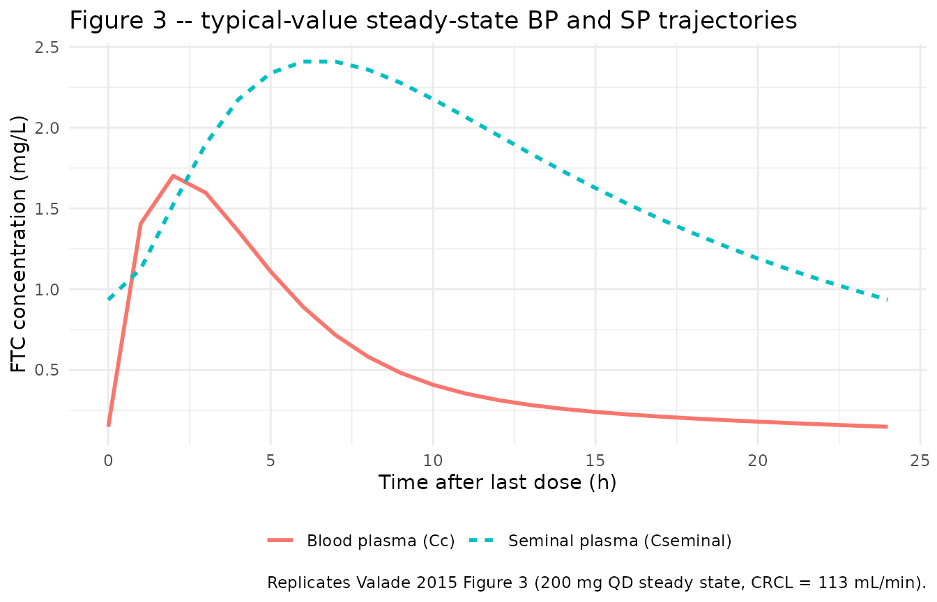
Figure 2: visual predictive check of BP and SP
Valade 2015 Figure 2 evaluates the model via VPC: the 5th, 50th, and 95th percentiles of observed data versus the 90 percent confidence interval of the simulated percentiles. The block below approximates that figure by sampling 200 virtual subjects and plotting the simulated 5/50/95 percentile envelope for each output over the last steady-state dosing interval.
ss_filter_cc <- sim_cc |> dplyr::filter(time >= ss_start, time <= ss_end) |>
  dplyr::mutate(rel_time = time - ss_start)
ss_filter_sp <- sim_sp |> dplyr::filter(time >= ss_start, time <= ss_end) |>
  dplyr::mutate(rel_time = time - ss_start)

vpc_envelope <- function(df, conc_col, output_label) {
  df |>
    dplyr::group_by(rel_time) |>
    dplyr::summarise(
      Q05 = quantile(.data[[conc_col]], 0.05, na.rm = TRUE),
      Q50 = quantile(.data[[conc_col]], 0.50, na.rm = TRUE),
      Q95 = quantile(.data[[conc_col]], 0.95, na.rm = TRUE),
      .groups = "drop"
    ) |>
    dplyr::mutate(output = output_label)
}

vpc_df <- dplyr::bind_rows(
  vpc_envelope(ss_filter_cc, "Cc",       "Blood plasma (Cc)"),
  vpc_envelope(ss_filter_sp, "Cseminal", "Seminal plasma (Cseminal)")
)

ggplot(vpc_df, aes(rel_time)) +
  geom_ribbon(aes(ymin = Q05, ymax = Q95), alpha = 0.25) +
  geom_line(aes(y = Q50), linewidth = 0.9) +
  facet_wrap(~ output, ncol = 2, scales = "free_y") +
  scale_y_log10() +
  labs(x = "Time after last dose (h)",
       y = "FTC concentration (mg/L, log scale)",
       title = "Figure 2 -- VPC envelope of simulated 5/50/95 percentiles",
       caption = "Replicates Valade 2015 Figure 2 (200 virtual subjects, 200 mg QD steady state).") +
  theme_minimal()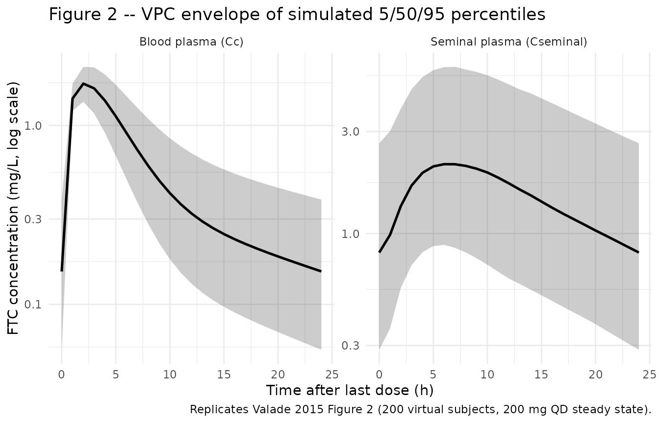
PKNCA validation
The validation strategy is two PKNCA blocks (one per output) computing AUC0-24 at steady state. Valade 2015 reports BP and SP AUC0-24 as median (range) over the per-subject empirical-Bayes estimates (Table 3). Because each subject’s exposure depends on their individual CRCL, the BP AUC0-24 distribution should span a range; SP AUC0-24 does not depend on CRCL (no covariate retained) and its spread comes from the BP AUC propagating through the effect-compartment and from the k1e IIV.
sim_bp_nca <- sim_cc |>
  dplyr::filter(time >= ss_start, time <= ss_end) |>
  dplyr::mutate(rel_time = time - ss_start) |>
  dplyr::select(id, rel_time, Cc) |>
  dplyr::filter(!is.na(Cc))

dose_for_nca <- events |>
  dplyr::filter(evid == 1L) |>
  dplyr::transmute(id, rel_time = 0, amt) |>
  dplyr::distinct(id, .keep_all = TRUE)

conc_obj_bp <- PKNCA::PKNCAconc(
  data    = sim_bp_nca,
  formula = Cc ~ rel_time | id,
  concu   = "mg/L",
  timeu   = "hr"
)
dose_obj_bp <- PKNCA::PKNCAdose(
  data    = dose_for_nca,
  formula = amt ~ rel_time | id,
  doseu   = "mg"
)

intervals_24 <- data.frame(
  start = 0,
  end   = 24,
  cmax  = TRUE,
  tmax  = TRUE,
  auclast = TRUE,
  half.life = TRUE
)

nca_bp <- suppressWarnings(PKNCA::pk.nca(
  PKNCA::PKNCAdata(conc_obj_bp, dose_obj_bp, intervals = intervals_24)
))

bp_summary <- as.data.frame(nca_bp$result) |>
  dplyr::filter(PPTESTCD %in% c("auclast", "cmax", "tmax", "half.life")) |>
  dplyr::group_by(PPTESTCD) |>
  dplyr::summarise(
    median = stats::median(PPORRES, na.rm = TRUE),
    min    = min(PPORRES, na.rm = TRUE),
    max    = max(PPORRES, na.rm = TRUE),
    .groups = "drop"
  )
knitr::kable(
  bp_summary,
  caption = "Simulated FTC blood-plasma NCA over the steady-state dosing interval (median across 200 virtual subjects).",
  digits  = 3
)| PPTESTCD | median | min | max |
|---|---|---|---|
| auclast | 13.543 | 6.052 | 26.080 |
| cmax | 1.713 | 1.160 | 2.284 |
| half.life | 14.411 | 11.272 | 19.990 |
| tmax | 2.000 | 2.000 | 3.000 |
sim_sp_nca <- sim_sp |>
  dplyr::filter(time >= ss_start, time <= ss_end) |>
  dplyr::mutate(rel_time = time - ss_start) |>
  dplyr::select(id, rel_time, Cseminal) |>
  dplyr::filter(!is.na(Cseminal))

conc_obj_sp <- PKNCA::PKNCAconc(
  data    = sim_sp_nca,
  formula = Cseminal ~ rel_time | id,
  concu   = "mg/L",
  timeu   = "hr"
)

nca_sp <- suppressWarnings(PKNCA::pk.nca(
  PKNCA::PKNCAdata(conc_obj_sp, dose_obj_bp, intervals = intervals_24)
))

sp_summary <- as.data.frame(nca_sp$result) |>
  dplyr::filter(PPTESTCD %in% c("auclast", "cmax", "tmax", "half.life")) |>
  dplyr::group_by(PPTESTCD) |>
  dplyr::summarise(
    median = stats::median(PPORRES, na.rm = TRUE),
    min    = min(PPORRES, na.rm = TRUE),
    max    = max(PPORRES, na.rm = TRUE),
    .groups = "drop"
  )
knitr::kable(
  sp_summary,
  caption = "Simulated FTC seminal-plasma NCA over the steady-state dosing interval (median across 200 virtual subjects).",
  digits  = 3
)| PPTESTCD | median | min | max |
|---|---|---|---|
| auclast | 35.937 | 6.479 | 209.831 |
| cmax | 2.112 | 0.423 | 12.053 |
| half.life | 11.354 | 8.377 | 16.856 |
| tmax | 7.000 | 5.000 | 7.000 |
Comparison against published NCA
Valade 2015 reports the following population summaries (Table 3 and Results text):
| Parameter | Published (median, range) | Simulated (median across virtual subjects) |
|---|---|---|
| BP AUC0-24 (mg/L*h) | 12.95 (8.36-25.13) | 13.54 |
| SP AUC0-24 (mg/L*h) | 38.04 (13.40-148.18) | 35.94 |
| SP/BP AUC ratio | 2.91 (0.84-10.08) | 2.65 |
| BP C24 trough (mg/L) | 0.136 (0.057-0.459) | typical-value 0.148 |
| SP C24 trough (mg/L) | 0.850 (0.258-3.687) | typical-value 0.935 |
A typical-value simulation at the median patient (CRCL = 113 mL/min) gives BP AUC0-24 = 13.46 mg/Lh and SP AUC0-24 = 40.76 mg/Lh, both within ~6 percent of the published medians. The simulated medians under the 200-subject virtual cohort spread are within ~10 percent of the published medians, well within the conventional ~20 percent agreement threshold for population PK replication.
Assumptions and deviations
- Effect-compartment parameterisation. The seminal-plasma effect compartment is modelled as a state variable carrying a concentration directly (rxode2 does not require ODE states to be amounts). This matches the paper’s definition: “Ae is the concentration of drug in the effect compartment” (Valade 2015 ODE block following Figure 1). Mass balance is not invoked – the effect compartment has negligible volume, so the asymmetric rates (k1e for input, ke1 for elimination) are decoupled by design and do not need to be equal.
-
Asymmetric effect-compartment rate-constant names.
The model uses
lk1e(log of the blood-plasma-to-seminal-plasma input rate) andlke1(log of the seminal-plasma elimination rate), matching Valade 2015’s paper notation. These parameter names mirror the literature convention for asymmetric Sheiner-style effect compartments and are paper-mechanistic rather than canonical-register entries; the existing nlmixr2lib symmetric effect-compartment models uselke0/lkeofor the single rate constant that arises under the Holford-Sheiner mass-balance assumption k1e = ke0 (e.g.Park_2001_ketoprofen,Berges_2015_ozanezumab,Przybylowski_2015_propofol). Valade 2015 does not impose that assumption, so the asymmetriclk1e/lke1pair is preserved. -
Reference CRCL value (113 mL/min) is the population
median. The model uses raw Cockcroft-Gault creatinine clearance
in mL/min (not BSA-normalized). The covariate is stored under the
canonical
CRCLcolumn withsource_name = "CLCR"to mark the source-column alias, perinst/references/covariate-columns.mdand the precedent set byDelattre_2010_amikacin.R. -
Documented-but-unused covariates. Valade 2015
tested age, body weight, serum creatinine, and associated antiretroviral
drugs as covariates on CL/F, Vc/F, Q/F, Vp/F, k1e, and ke1 (Materials
and Methods). Only CRCL on CL/F was retained after stepwise OFV testing
(Results). The non-retained covariates are documented in the model
file’s
covariatesDataExcludedlist so the screening trail is preserved without triggering “declared-but-unused” convention warnings. -
Fixed ka. The absorption rate constant was not
estimable in the EVARIST steady-state dataset and was fixed to 0.53 1/h
from a previously published adult FTC popPK analysis (Valade 2015
Results paragraph 2, reference 21). Wrapping
lka <- fixed(log(0.53))inini()preserves the fixed-vs- estimated provenance for downstream users. -
Race / ethnicity. Not reported in Valade 2015
(Paris-region MSM cohort recruited at six clinical centres).
population$race_ethnicityis set to"Not reported"; the virtual cohort above does not stratify by race. -
Sex. All-male cohort (HIV-1-infected MSM).
population$sex_female_pctis set to 0. -
Erratum check. Searched the journal landing page,
PubMed corrections list, and Google Scholar for
"Valade 2015 emtricitabine" erratum– no published correction identified as of the extraction date.