Linagliptin DPP-4 TMDD-PBPK: whole-body distribution and renal reabsorption (Nakamura 2024)
Source:vignettes/articles/Nakamura_2024_linagliptin_pbpk.Rmd
Nakamura_2024_linagliptin_pbpk.RmdModel and source
- Citation: Nakamura R, Yoshikado T, Aoki Y, Sugiyama Y, Chiba K. Elucidation of DPP-4 involvement in systemic distribution and renal reabsorption of linagliptin by PBPK modeling with a cluster Gauss-Newton method. Clin Transl Sci. 2024;17(10):e70047. doi:10.1111/cts.70047. The ODE system is transcribed from the deposited human model code (Data S2, Program/pbpk_lng_human/lng_pbpk_model_human.r); the estimated parameters are the median column of Table 2 and the fixed physiological parameters are Table S2 and the deposited paramdata.
- Article: https://doi.org/10.1111/cts.70047 (open access, PMC11494486)
- Supporting Information published with the article: Data S1
(Supplementary Text, Tables S1-S7, Figures S1-S7) and Data S2, the
authors’ complete rat and human model code in
d/dt()form, from which the ODE systems in this package are transcribed.
Linagliptin (LNG) is a dipeptidyl peptidase-4 (DPP-4) inhibitor with strongly nonlinear pharmacokinetics: plasma exposure rises faster than dose and urinary excretion is dose-dependent. The cause is target-mediated drug disposition (TMDD) against DPP-4, which linagliptin binds with sub-nanomolar affinity. Nakamura et al. build a whole-body physiologically based pharmacokinetic (PBPK) model in which DPP-4 is carried explicitly in every organ as two species – soluble plasma DPP-4 (sDPP-4) and transmembrane tissue DPP-4 (tDPP-4) – and linagliptin binds both reversibly with a time-dependent on/off kinetic (kon = koff / Kd). Two consequences of binding drive the nonlinearity:
- Saturable plasma protein binding to sDPP-4 makes dose-normalised unbound AUC roughly constant while total exposure rises more than proportionally.
- DPP-4-complex-mediated renal reabsorption: the linagliptin-tDPP-4 complex formed in the renal tubule is reabsorbed at a constant clearance (CLreab,DPP4). Because complex formation saturates, so does reabsorption, which the authors show is necessary to reproduce the dose-dependent urinary excretion – a model with CLreab,DPP4 fixed to zero, or with reabsorption of unbound drug only, cannot.
The parameters are estimated with the cluster Gauss-Newton method
(CGNM), a multi-start nonlinear least-squares method that returns an
ensemble of accepted parameter combinations rather than a single fit.
The rat tissue DPP-4 distribution (from [14C]-linagliptin
autoradiography in wild-type and Dpp-4-deficient rats) is estimated
first and carried into the human model as fixed tissue DPP-4
concentration ratios.
Models in this package
The package ships the two models whose published CGNM ensembles reconstitute their reported fits from the tabulated marginal medians:
-
Nakamura_2024_linagliptin_human_pbpk– the human model (Table 2), 112 ODE states. -
Nakamura_2024_linagliptin_rat_pbpk– the rat whole-body (plasma- concentration) model (plasma column of Table 1), 92 ODE states. The Dpp-4-deficient rat is reproduced by setting the total DPP-4 amount to zero.
Both carry DPP-4 (free and complexed) and linagliptin as separate
states in every organ; the state names are kept verbatim from Data S2 so
the ODEs can be checked line-by-line against the authors’ code (they are
declared as paper_specific_compartments).
hmod <- readModelDb("Nakamura_2024_linagliptin_human_pbpk")
rmod <- readModelDb("Nakamura_2024_linagliptin_rat_pbpk")
hui <- rxode2::rxode2(hmod)
length(hui$state)
#> [1] 112
Population
readModelDb("Nakamura_2024_linagliptin_human_pbpk")()$population$notes
#> [1] "The human clinical data (plasma concentration, urinary and faecal excretion after intravenous and oral linagliptin) are the pooled healthy-volunteer data of Sarashina 2010 / Retlich 2010 / Blech 2010, the same data analysed in Sarashina 2020. Individual subject counts, ages, weights and sex are not reported by Nakamura 2024; all physiological parameters are scaled to a single typical 70 kg adult. Doses are supplied in nmol (linagliptin MW 472.54; the deposited code converts mg to nmol with the factor 2116.22 nmol/mg)."
The human clinical data are the pooled healthy-volunteer intravenous
(0.5-10 mg, 1.5 h infusion) and oral (1-10 mg) linagliptin studies
analysed in Sarashina 2020. The rat data are
[14C]-linagliptin plasma concentrations in wild-type and
Dpp-4-deficient rats (Retlich 2009) plus autoradiography tissue and
excretion data (Fuchs 2009). The models are deterministic (CGNM is a
fixed-effects method): there is no between-subject variability, so a
single typical-value rxSolve() is the whole prediction.
Source trace
Every parameter value carries an in-file comment pointing to its source. The structural parameters below are the CGNM medians; all physiological constants are fixed from the supplementary tables and the deposited parameter data.
| Source | Content |
|---|---|
| Table 2 (medians) | the 16 estimated human parameters (CLint,h, CLsec,int, CLreab,DPP4, AsDPP4, AtDPP4, Kd, koff, Vmax,P-gp, PSdif,ent,BE, LR, rAlpha, Kp,rem, fbile, flumen,gut, flumen,kidney, rGL) |
| Table 1, plasma column (medians) | the 16 estimated rat parameters; ADPP4 = AsDPP4 (0.0312 nmol) / fsDPP4 (0.001976) = 15.79 nmol |
| Table S2 | human physiological volumes, blood flows, partition coefficients, fup, RB |
| Table S1 | rat physiological parameters |
| Data S2 | tissue DPP-4 concentrations / fractions (rat autoradiography), segmented-flow intestine fractions, transit rate constants |
| Table S6 | non-compartmental AUC/Dose and CLR,u by intravenous dose (the nonlinearity this vignette checks) |
The equation forms (reversible DPP-4 binding, Eqs 1-2; DPP-4-complex renal reabsorption, Eq 3) are transcribed from Data S2.
Human model: nonlinear plasma pharmacokinetics (replicates Figure 3)
nmolf <- 2116.22 # nmol per mg linagliptin (MW 472.54); deposited conversion factor

# Intravenous arms: 1.5 h infusion into blood (ABlood). Oral arms: bolus into
# the duodenal lumen.
iv_doses <- c(0.5, 2.5, 5, 10)
po_doses <- c(1, 2.5, 5, 10)

# Gastrointestinal-motility inhibition (GIMI = 1) lasts until the colon mean
# residence time, which the authors set per dose level (Supplementary Text).
# Their event table keys the window on the dose alone, so it applies to the
# intravenous arms too; the 0.5 mg arm has no window (GIMI = 0 throughout).
mrt_colon <- c(`0.5` = 0, `1` = 2.00, `2.5` = 5.23, `5` = 10.6, `10` = 18.4)

tgrid <- sort(unique(c(seq(0, 6, by = 0.05), seq(6, 24, by = 0.25),
                       seq(24, 196, by = 1))))

solve_arm <- function(dose, route) {
  ev <- if (route == "intravenous") {
    rxode2::et(amt = nmolf * dose, cmt = "ABlood", dur = 1.5)
  } else {
    rxode2::et(amt = nmolf * dose, cmt = "Aduodenum_lumen")
  }
  ev <- as.data.frame(rxode2::et(ev, tgrid))
  ev$GIMI <- as.integer(ev$time < mrt_colon[[as.character(dose)]])
  s <- rxode2::rxSolve(hmod, ev, returnType = "data.frame", atol = 1e-9, rtol = 1e-7)
  s$dose_mg <- dose
  s$route <- route
  s
}

hsim <- dplyr::bind_rows(
  lapply(iv_doses, solve_arm, route = "intravenous"),
  lapply(po_doses, solve_arm, route = "oral")
)
# Observed plasma concentrations (nmol/L), a subset of time points transcribed
# from the authors' deposited analysis dataset (Data S2, lngdata_human.rdata).
obs_iv <- tibble::tribble(
  ~dose_mg, ~time, ~Value,
  0.5, 2, 5.778, 0.5, 6, 3.876, 0.5, 24, 2.646, 0.5, 72, 1.533,
  5, 2, 39.078, 5, 6, 19.568, 5, 24, 6.874, 5, 72, 4.452,
  10, 2, 69.348, 10, 6, 29.462, 10, 24, 8.95, 10, 72, 3.81
) |> dplyr::mutate(route = "intravenous")
obs_po <- tibble::tribble(
  ~dose_mg, ~time, ~Value,
  1, 1.5, 4.32, 1, 6, 3.426, 1, 24, 1.971, 1, 72, 0.961,
  5, 3, 7.212, 5, 8, 8.458, 5, 24, 5.602, 5, 72, 3.187,
  10, 2, 16.164, 10, 8, 13.909, 10, 24, 7.117, 10, 72, 3.805
) |> dplyr::mutate(route = "oral")
hobs <- dplyr::bind_rows(obs_iv, obs_po)
# Plotting frame only: the near-zero values in the first minutes after an oral
# dose would otherwise stretch the log axis over five decades.
prof <- hsim[hsim$time <= 72 & hsim$Cc > 0.1, ]
ggplot(prof, aes(time, Cc, colour = factor(dose_mg))) +
  geom_line() +
  geom_point(data = hobs, aes(time, Value, colour = factor(dose_mg)), size = 1.6) +
  facet_wrap(~route) +
  scale_y_log10() +
  labs(x = "Time (h)", y = "Plasma linagliptin (nmol/L)", colour = "Dose (mg)",
       title = "Human linagliptin, model lines vs observed points (Figure 3)") +
  theme_bw()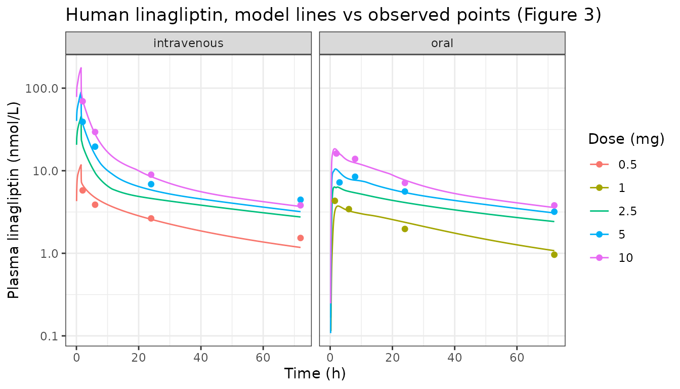
The lines are the typical-value PBPK prediction; the points are observed plasma concentrations. Across both routes the model tracks the more-than-dose- proportional rise and the long terminal phase that DPP-4 binding produces.
Human nonlinearity check against the non-compartmental analysis (Table S6)
The paper’s non-compartmental analysis (Table S6) reports that dose-normalised total AUC falls with dose over the intravenous range – the signature of saturable DPP-4 binding. We reproduce the NCA on the simulated intravenous profiles with PKNCA and compare.
iv <- hsim[hsim$route == "intravenous", ]
# PKNCA needs a time-zero record; the infusion starts at 0 so Cc(0) = 0.
conc <- iv |>
  dplyr::transmute(dose_mg, time, Cc) |>
  dplyr::filter(!is.na(Cc)) |>
  dplyr::mutate(treatment = paste0(dose_mg, " mg iv"))

dose_df <- conc |>
  dplyr::group_by(treatment, dose_mg) |>
  dplyr::summarise(time = 0, .groups = "drop") |>
  dplyr::mutate(dose_nmol = nmolf * dose_mg)

o_conc <- PKNCA::PKNCAconc(conc, Cc ~ time | treatment)
o_dose <- PKNCA::PKNCAdose(dose_df, dose_nmol ~ time | treatment)
intervals <- data.frame(start = 0, end = Inf, aucinf.obs = TRUE, cmax = TRUE)
res <- PKNCA::pk.nca(PKNCA::PKNCAdata(o_conc, o_dose, intervals = intervals))

nca <- as.data.frame(res$result) |>
  dplyr::filter(PPTESTCD == "aucinf.obs") |>
  dplyr::left_join(dplyr::distinct(dose_df, treatment, dose_mg, dose_nmol), by = "treatment") |>
  # Table S6 normalises total AUC (nmol*h/L) by the dose in nmol.
  dplyr::mutate(auc_over_dose = PPORRES / dose_nmol) |>
  dplyr::arrange(dose_mg)

# Table S6 reported total AUC/Dose = AUC (nmol*h/L) / Dose (nmol), intravenous:
ts6 <- c(`0.5` = 0.4082, `2.5` = 0.1558, `5` = 0.1192, `10` = 0.0727)

cmp <- nca |>
  dplyr::transmute(
    dose_mg,
    `AUC/Dose simulated` = round(auc_over_dose, 4),
    `AUC/Dose Table S6` = ts6[as.character(dose_mg)]
  )
knitr::kable(cmp, caption = "Dose-normalised total plasma AUC: simulated vs Table S6.")| dose_mg | AUC/Dose simulated | AUC/Dose Table S6 |
|---|---|---|
| 0.5 | 0.4247 | 0.4082 |
| 2.5 | 0.1600 | 0.1558 |
| 5.0 | 0.1000 | 0.1192 |
| 10.0 | 0.0680 | 0.0727 |
sim_od <- nca$auc_over_dose
names(sim_od) <- as.character(nca$dose_mg)
# 1. The nonlinearity has the right sign and magnitude: dose-normalised AUC
#    falls several-fold from the lowest to the highest intravenous dose. Table
#    S6 gives a 5.6-fold drop (0.408 -> 0.073).
fold_obs <- ts6["0.5"] / ts6["10"]
fold_sim <- sim_od["0.5"] / sim_od["10"]
stopifnot(
  fold_sim > 2,                              # strongly nonlinear
  abs(log(fold_sim / fold_obs)) < log(1.6)   # within ~1.6-fold of the reported drop
)
# 2. Each simulated dose-normalised AUC is within 2-fold of Table S6.
stopifnot(all(abs(log(sim_od / ts6[names(sim_od)])) < log(2)))
c(fold_simulated = unname(round(fold_sim, 2)), fold_TableS6 = unname(round(fold_obs, 2)))
#> fold_simulated   fold_TableS6
#>           6.24           5.61
Rat model: DPP-4 deficiency abolishes the DPP-4-dependent disposition (replicates Figure 1f)
In Dpp-4-deficient rats the drug has no high-affinity binding sites,
so plasma declines faster and the DPP-4-mediated prolongation of
exposure disappears. The deficient animal is simulated by driving the
total DPP-4 amount to zero (lADPP4 on the log scale).
BW <- 0.25 # kg, body weight of the rat
rmod_def <- rmod |> rxode2::ini(lADPP4 = log(1e-9))
#> ℹ change initial estimate of `lADPP4` to `-20.7232658369464`

rgrid <- sort(unique(c(seq(0, 8, by = 0.1), seq(8, 72, by = 0.5))))
solve_rat <- function(model, dose_mgkg, strain) {
  ev <- rxode2::et(amt = nmolf * dose_mgkg * BW, cmt = "ABlood") |>
    rxode2::et(rgrid)
  s <- rxode2::rxSolve(model, ev, returnType = "data.frame", atol = 1e-9, rtol = 1e-7)
  s$dose_mgkg <- dose_mgkg
  s$strain <- strain
  s
}

rsim <- dplyr::bind_rows(
  solve_rat(rmod, 1, "wild-type"), solve_rat(rmod_def, 1, "Dpp-4 deficient"),
  solve_rat(rmod, 10, "wild-type"), solve_rat(rmod_def, 10, "Dpp-4 deficient")
)

# Observed plasma concentrations (nmol/L) from the authors' deposited rat
# dataset (Data S2, lngdata_rat.rdata; Retlich 2009). The 72 h deficient
# samples were below the limit of quantification.
robs <- tibble::tribble(
  ~strain, ~dose_mgkg, ~time, ~Value,
  "wild-type", 1, 1, 78.855, "wild-type", 1, 4, 19.231, "wild-type", 1, 8, 6.694,
  "wild-type", 1, 24, 2.16, "wild-type", 1, 48, 3.381, "wild-type", 1, 72, 0.791,
  "Dpp-4 deficient", 1, 1, 80.492, "Dpp-4 deficient", 1, 4, 12.499,
  "Dpp-4 deficient", 1, 8, 2.804, "Dpp-4 deficient", 1, 24, 0.415, "Dpp-4 deficient", 1, 48, 0.113,
  "wild-type", 10, 1, 1327.99, "wild-type", 10, 4, 416.04, "wild-type", 10, 8, 82.18,
  "wild-type", 10, 24, 8.204, "wild-type", 10, 48, 3.858, "wild-type", 10, 72, 1.87,
  "Dpp-4 deficient", 10, 1, 1827.01, "Dpp-4 deficient", 10, 4, 336.13,
  "Dpp-4 deficient", 10, 8, 52.52, "Dpp-4 deficient", 10, 24, 7.925, "Dpp-4 deficient", 10, 48, 0.752
)
# Plotting frame only: drop the bolus instant, whose 1e5 nmol/L spike would
# compress the axis.
rprof <- rsim[rsim$time >= 0.5 & rsim$Plasma > 0, ]
ggplot(rprof, aes(time, Plasma, colour = strain)) +
  geom_line() +
  geom_point(data = robs, aes(time, Value, colour = strain), size = 1.6) +
  facet_wrap(~dose_mgkg, labeller = labeller(dose_mgkg = c(`1` = "1 mg/kg", `10` = "10 mg/kg"))) +
  scale_y_log10() +
  labs(x = "Time (h)", y = "Plasma linagliptin (nmol/L)", colour = "Strain",
       title = "Rat linagliptin, wild-type vs Dpp-4 deficient (Figure 1f)") +
  theme_bw()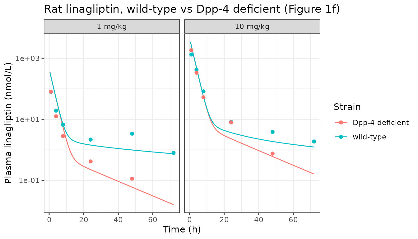
# The mechanistic signature: in the terminal phase the Dpp-4-deficient rat has
# lower plasma than the wild-type at the same dose, because DPP-4 binding is
# what sustains wild-type exposure. Check at 24 h for both doses.
term <- rsim[rsim$time == 24, c("dose_mgkg", "strain", "Plasma")]
wt24 <- term$Plasma[term$strain == "wild-type"]
def24 <- term$Plasma[term$strain == "Dpp-4 deficient"]
stopifnot(all(def24 < wt24))                       # deficiency lowers terminal exposure
stopifnot(all(is.finite(rsim$Plasma)))             # no integration failure
round(data.frame(dose_mgkg = c(1, 10), wt_24h = wt24, def_24h = def24), 3)
#>   dose_mgkg wt_24h def_24h
#> 1         1  1.428   0.224
#> 2        10  3.653   2.302
Assumptions and deviations (Errata)
-
No between-subject variability or residual error.
CGNM is a fixed-effects nonlinear-least-squares method; the paper
reports neither an IIV nor a residual-error model. Each
propSdis afixed(0.1)placeholder so the model object carries a residual slot, and the models are used as typical-value predictors. -
GIMIis a paper-specific covariate, not a canonical register name. The gastrointestinal-motility-inhibition indicator (1 while a dose is within its colon mean-residence-time window, scaling the intestinal transit rate constants byrAlpha) is a time-varying structural switch the authors encode per record; it is not ininst/references/covariate-columns.mdandcheckModelConventions()flags it as non-canonical. SetGIMI = 1for records withtime < MRTcolon(2.00, 5.23, 10.6 and 18.4 h for 1, 2.5, 5 and 10 mg) andGIMI = 0otherwise. The authors’ event table keys this window on the dose level only, so it applies to the intravenous 2.5-10 mg arms as well as the oral arms; the 0.5 mg arm has no window. The window is defined only for these four single doses, so a simulation of another dose or of repeated dosing has to choose its ownGIMIpattern. - Doses are supplied in nmol. Linagliptin MW is 472.54 g/mol; the deposited code converts mg to nmol with 2116.22 nmol/mg, which this vignette reuses.
-
The rat autoradiography tissue-distribution analysis is not
shipped as a separate model. CGNM publishes only the marginal
quantiles of its accepted ensemble (Table 1), not the joint best-fit
parameter vector, and for the autoradiography analysis the
marginal-median vector does not reconstitute the reported fit (its sum
of squared residuals is several-fold worse than the reported ensemble
median). Its scientific output – the tissue DPP-4 concentration ratios
and the estimated liver/reproductive-organ/salivary-gland Kp
values – is instead carried as fixed parameters in both shipped models
(the
CDPP4_*/fDPP4_*andKp*_vivoconstants), so nothing from that analysis is lost. - Low-dose rat early time points. With the Table 1 marginal-median parameter vector the rat model over-predicts the first hours of the low-dose arms; the authors describe their rat plasma fit as “roughly reproducing” the data (reported plasma-model SSR ensemble 12.0-15.3). The higher-dose arms and the deficiency contrast, which carry the mechanism, track well.
-
Table 1
f bile(rat autoradiography column) is anomalous (median 101 for a quantity the model constrains to the unit interval); it is not used here because the autoradiography model is not shipped.