SR9009 lung circadian clock and SARS-CoV-2 QSP model (Tseng 2025)
Source:vignettes/articles/Tseng_2025_SR9009.Rmd
Tseng_2025_SR9009.RmdModel and source
Tseng 2025 builds a theoretical quantitative systems pharmacology model of the circadian clock in a lung cell and couples it to SARS-CoV-2 infection. The clock drives the viral entry receptor ACE2 (through CLOCK:BMAL1) and represses interferon-stimulated genes (ISG), so the infection oscillates with the clock. The REV-ERB agonist SR9009, which represses Bmal1 through REV-ERB, is then given as a once-daily 1 h exposure at different circadian times to look for a dosing time that suppresses the virus while keeping the clock running.
mod <- rxode2::rxode(readModelDb("Tseng_2025_SR9009_qsp"))- Citation: Tseng Y-Y. (2025). A theoretical systems chronopharmacology approach for COVID-19: Modeling circadian regulation of lung infection and potential precision therapies. CPT Pharmacometrics Syst Pharmacol 14(2):340-350. doi:10.1002/psp4.13277. Equations from Data S1, parameter values from Table S1, and initial conditions, inoculum, SR9009 and cortisol switch values from the SBML model deposited as File S1.
- Description: QSP. Theoretical (in silico) lung-cell circadian clock model coupled to SARS-CoV-2 entry and replication, with the REV-ERB agonist SR9009 as a timed perturbation (Tseng 2025). Twelve clock ODEs (Per/Cry, Clock/Bmal1, Dbp, Ror and Rev-Erb mRNAs and proteins, plus the PER:CRY and CLOCK:BMAL1 complexes) with Hill-type transcriptional activation and repression and first-order degradation give a free-running 24 h oscillator. Four infection ODEs couple to it: ACE2 (induced by CLOCK:BMAL1, repressed by PER:CRY) gates entry of free virus into the endosome, endosomal virus cycles with replicated virus, and interferon-stimulated genes (ISG; repressed by CLOCK:BMAL1, induced by PER:CRY) repress replication. SR9009 adds a zero-order term to Rev-Erb transcription while a dose is on; a cortisol pulse adds to Per/Cry transcription and blocks Rev-Erb transcription. Inoculation, SR9009 and cortisol exposures are given as events: a dose of 1 into vfree inoculates, and a dose of 1 into sr9009 or cortisol switches the exposure on until a replacement (evid = 5, amt = 0) event switches it off. All levels are in arbitrary units and time in hours. Deterministic: no between-subject variability and no residual error.
- Article: https://doi.org/10.1002/psp4.13277
- PubMed Central: https://www.ncbi.nlm.nih.gov/pmc/articles/PMC11812942/
The equations are printed in Data S1 and the parameter values in
Table S1. The author also deposited the CellDesigner model in SBML (File
S1), which carries the initial conditions, the virus-entry rate
kin_Vfree, and the event switches used for the inoculation,
the SR9009 doses and the cortisol pulses; two Python scripts (robustness
and sensitivity analysis) run a reduced copy of that SBML file.
Population
There is no study population. The model is a single in silico lung epithelial cell, with all levels in arbitrary units and time in hours. The mRNA degradation rates were taken from experimental data or published models and the remaining parameters and initial conditions were tuned by hand until the clock oscillated with a 24 h period and the mRNA peak phases fell in the experimental windows of Figure 2b. The infection layer was matched qualitatively to the BMAL1 / ACE2 / ISG findings of Zhuang et al. (2021) in Calu-3 lung epithelial cells. SR9009 has no pharmacokinetic model: its exposure is the on/off level of a term added to Rev-Erb transcription.
The same information is available programmatically via
readModelDb("Tseng_2025_SR9009_qsp")()$population.
How the model is driven
Three inputs are given as events, each on its own state:
| Input | State | On | Off |
|---|---|---|---|
| SARS-CoV-2 inoculation | vfree |
dose amt = 1
|
(stays on) |
| SR9009 exposure | sr9009 |
dose amt = 1
|
replacement evid = 5, amt = 0
|
| Cortisol pulse | cortisol |
dose amt = 1
|
replacement evid = 5, amt = 0
|
The SBML file does the same thing with event assignments:
Vfree is set to 1 at 24 h, Ka_rev_SR9009 is
switched between 0 and 0.5, and the cortisol parameters between their
resting and pulse values. Circadian time (CT) is the model time modulo
24 h: Figure 5 states that SR9009 at CT 18 starts at 66 h.
# Observation grid on an ODE state; the algebraic outputs (total_virus) are
# returned as columns at every observation row.
obs_grid <- function(end = 200, by = 0.1) {
  data.frame(id = 1L, time = seq(0, end, by = by), evid = 0L, amt = 0, cmt = "pc_mrna")
}

# Inoculation at 24 h (File S1 'Virus_on': T_virus_on = 24, Vfree_on = 1).
inoculate <- function(time = 24) {
  data.frame(id = 1L, time = time, evid = 1L, amt = 1, cmt = "vfree")
}

# A switch held on from `on` to `on + dur` for each start time.
pulse <- function(cmt, on, dur = 1) {
  rbind(
    data.frame(id = 1L, time = on, evid = 1L, amt = 1, cmt = cmt),
    data.frame(id = 1L, time = on + dur, evid = 5L, amt = 0, cmt = cmt)
  )
}

solve_events <- function(model, ev, ...) {
  ev <- dplyr::arrange(ev, time, dplyr::desc(evid))
  as.data.frame(rxode2::rxSolve(model, ev, rtol = 1e-10, atol = 1e-10, ...))
}

# Local maxima / minima of a sampled curve.
peaks <- function(t, x) {
  i <- which(diff(sign(diff(x))) == -2) + 1
  data.frame(time = t[i], value = x[i])
}
troughs <- function(t, x) {
  i <- which(diff(sign(diff(x))) == 2) + 1
  data.frame(time = t[i], value = x[i])
}
Source trace
| Model element | Source location |
|---|---|
Clock mRNA ODEs (cb_mrna, pc_mrna,
dbp_mrna, ror_mrna,
rev_mrna) |
Data S1 Eqs. 1-5; SBML reactions re10, re44, re40, re22, re21 |
| Clock protein and complex ODEs | Data S1 Eqs. 6-12 |
| ACE2, endosomal virus, replicated virus, ISG ODEs | Data S1 Eqs. 13-16 |
| Free virus as a non-depleted input | Data S1 (four ODEs added; [Vfree] appears only as a
driver); Figure 5a |
| Transcription, translation, complex-formation, threshold, Hill and degradation constants | Table S1 |
kin_vfree = 0.3 |
File S1 (SBML global parameter kin_Vfree; absent from
Table S1) |
ace2_mrna = 1, isg_pre = 1 |
File S1 (boundary species ace2_RNA,
ISGpre) |
ka_rev_sr9009 = 0.5, 1 h per dose |
File S1 (Ka_rev_SR9009_on = 0.5, SP = 1);
Figure 5b right axis; Results text |
kact_pc_cortisol = 10, krep_rev_cortisol =
0, 1 h pulse |
Methods ‘Modeling cortisol pulses’; File S1
(kact_pc_cortisol_on, Krep_rev_cortisol_on,
CP = 1) |
| Initial conditions of the 14 clock / infection states | File S1 (species initialAmount) |
total_virus = vendo + vrep |
File S1 assignment rule total_virus; plotted as
‘SARS-CoV-2’ in Figure 5 and ‘Total Virus’ in Figure S8 |
The parameter values are checked against a transcription of Table S1 (and of the File S1 values for the parameters Table S1 omits):
table_s1 <- c(
  ktx_cb = 0.55, ktx_dbp = 1.24, ktx_pc = 3.9, ktx_rev = 1.15, ktx_ror = 0.29,
  ktl_cb = 0.6, ktl_dbp = 0.7, ktl_pc = 0.5, ktl_rev = 0.6, ktl_ror = 0.3,
  kf_cbc = 0.3, kf_pcc = 0.5,
  ka_cb_ror = 0.85, ka_dbp_cbc = 1, ka_pc_cbc = 0.3, ka_pc_dbp = 0.5,
  ka_pc_ror = 1.85, ka_rev_cbc = 0.85, ka_rev_dbp = 0.1, ka_ror_dbp = 0.33,
  ki_cb_rev = 0.6, ki_dbp_pcc = 0.6, ki_pc_pcc = 1, ki_pc_rev = 4, ki_rev_pcc = 0.8,
  hill_cb_rev = 4, hill_cb_ror = 2, hill_dbp_cbc = 4, hill_dbp_pcc = 2,
  hill_pc_cbc = 2, hill_pc_dbp = 2, hill_pc_pcc = 4, hill_pc_rev = 4,
  hill_pc_ror = 4, hill_rev_cbc = 4, hill_rev_dbp = 2, hill_rev_pcc = 2,
  hill_ror_dbp = 2,
  kdeg_cb_mrna = 0.37, kdeg_dbp_mrna = 0.36, kdeg_pc_mrna = 0.3,
  kdeg_rev_mrna = 0.55, kdeg_ror_mrna = 0.31, kdeg_cb_prot = 0.2,
  kdeg_dbp_prot = 0.3, kdeg_pc_prot = 0.3, kdeg_rev_prot = 0.25,
  kdeg_ror_prot = 0.18, kdeg_cbc = 0.27, kdeg_pcc = 0.3,
  ktl_ace2 = 0.25, k_isg = 0.3, k_vendo = 0.5, k_vrep = 5,
  ka_ace2_cbc = 0.3, ka_isg_pcc = 0.01, ka_vin_ace2 = 0.3, ki_ace2_pcc = 2.4,
  ki_isg_cbc = 1, ki_vrep_isg = 1, hill_ace2_cbc = 4, hill_ace2_pcc = 2.01,
  hill_isg_cbc = 2, hill_isg_pcc = 2, hill_vin_ace2 = 2, hill_vrep_isg = 2,
  kdeg_ace2 = 0.3, kdeg_isg = 0.3, kdeg_vendo = 3.164
)
file_s1 <- c(
  kin_vfree = 0.3, ace2_mrna = 1, isg_pre = 1,
  ka_rev_sr9009 = 0.5, kact_pc_cortisol = 10, krep_rev_cortisol = 0
)
expected <- c(table_s1, file_s1)
theta <- mod$theta
stopifnot(
  setequal(names(theta), names(expected)),
  isTRUE(all.equal(theta[names(expected)], expected, tolerance = 1e-12))
)
length(expected)
#> [1] 75
Free-running clock (Figure 2)
sim_clock <- solve_events(mod, obs_grid(end = 200, by = 0.01))

clock_long <- sim_clock |>
  dplyr::filter(time <= 50) |>
  dplyr::select(time, cb = cb_mrna, Dbp = dbp_mrna, pc = pc_mrna, `Rev-Erb` = rev_mrna, Ror = ror_mrna) |>
  tidyr::pivot_longer(-time, names_to = "mRNA", values_to = "level")
ggplot(clock_long, aes(time, level, colour = mRNA)) +
  geom_line(linewidth = 0.8) +
  labs(x = "Time (h)", y = "RNA level (a.u.)", colour = NULL) +
  theme_bw()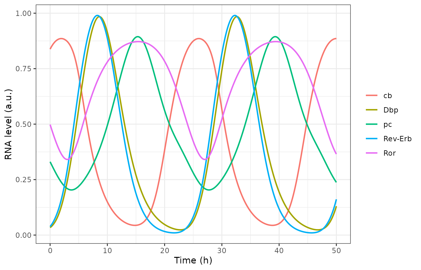
Replicates Figure 2a of Tseng 2025: clock mRNA oscillations of the free-running model.
Figure 2b compares the simulated peak time of each mRNA (black dots) with the window in which the measured mRNA is above 70% of its peak (colour bands, read from the figure). The simulated peaks are taken from the fifth cycle so that they are on the limit cycle:
peak_ct <- function(x) {
  p <- peaks(sim_clock$time, x)
  p <- p[p$time >= 96 & p$time < 120, ]
  p$time[1] %% 24
}
phase <- tibble::tibble(
  mRNA = c("Bmal (cb)", "Dbp", "Per2 (pc)", "Rora", "Rev"),
  sim_ct = c(
    peak_ct(sim_clock$cb_mrna), peak_ct(sim_clock$dbp_mrna),
    peak_ct(sim_clock$pc_mrna), peak_ct(sim_clock$ror_mrna),
    peak_ct(sim_clock$rev_mrna)
  ),
  # Figure 2b: shaded CT cells (window start, window end + 1 h) and the
  # simulated peak dot, read by the maintainers.
  window_lo = c(0, 8, 11, 8, 8),
  window_hi = c(3, 14, 17, 21, 14),
  paper_dot = c(2, 9, 15, 15, 8)
)
phase |>
  dplyr::mutate(sim_ct = round(sim_ct, 1)) |>
  dplyr::rename(
    "mRNA" = mRNA, "Simulated peak (CT, h)" = sim_ct,
    "Window start (CT)" = window_lo, "Window end (CT)" = window_hi,
    "Figure 2b dot (CT)" = paper_dot
  ) |>
knitr::kable(caption = "Peak phases of the clock mRNAs against Figure 2b.")| mRNA | Simulated peak (CT, h) | Window start (CT) | Window end (CT) | Figure 2b dot (CT) |
|---|---|---|---|---|
| Bmal (cb) | 2.0 | 0 | 3 | 2 |
| Dbp | 8.7 | 8 | 14 | 9 |
| Per2 (pc) | 15.4 | 11 | 17 | 15 |
| Rora | 15.5 | 8 | 21 | 15 |
| Rev | 8.3 | 8 | 14 | 8 |
stopifnot(
  all(phase$sim_ct >= phase$window_lo & phase$sim_ct < phase$window_hi),
  all(abs(phase$sim_ct - phase$paper_dot) < 1)
)
The state at the start of the simulation is a point on the limit cycle, so the oscillation neither decays nor grows and the model returns to the same state one period later:
pk_pc <- peaks(sim_clock$time, sim_clock$pc_mrna)
period <- diff(pk_pc$time)
amp <- range(pk_pc$value)
c(min_period = min(period), max_period = max(period), min_peak = amp[1], max_peak = amp[2])
#> min_period max_period   min_peak   max_peak
#> 24.0100000 24.0200000  0.8941435  0.8941451
stopifnot(all(abs(period - 24) < 0.1), diff(amp) < 1e-3)
Sensitivity of period and amplitude (Figures S3-S4)
The paper reports local response coefficients from a 3% perturbation
of each parameter, averaged over the increase and the decrease, with the
period and amplitude of pc_RNA taken from a 200 h
simulation sampled every 0.005 h (the deposited script
PSP-2024-0047-s06.py). The period is the mean of the last
two peak-to-peak intervals and the amplitude is the last peak minus the
trough before it. Four of the coefficients are quoted in the Results
text.
clock_metrics <- function(params) {
  s <- solve_events(mod, obs_grid(end = 200, by = 0.005), params = params)
  p <- peaks(s$time, s$pc_mrna)
  n <- nrow(p)
  period <- mean(diff(p$time)[(n - 2):(n - 1)])
  last <- s$time >= p$time[n - 1] & s$time <= p$time[n]
  amplitude <- p$value[n] - min(s$pc_mrna[last])
  c(period = period, amplitude = amplitude)
}
base_metrics <- clock_metrics(theta)
response_coefficient <- function(par, delta = 0.03) {
  up <- theta
  up[[par]] <- up[[par]] * (1 + delta)
  dn <- theta
  dn[[par]] <- dn[[par]] * (1 - delta)
  ((clock_metrics(up) - base_metrics) / base_metrics / delta +
    (clock_metrics(dn) - base_metrics) / base_metrics / (-delta)) / 2
}
rc_check <- tibble::tibble(
  parameter = c("kdeg_cb_mrna", "kdeg_cbc", "ktx_ror", "ktl_ror"),
  paper_name = c("kd_cb", "kd_CBC", "k_ror", "k_ROR"),
  output = c("period", "period", "amplitude", "amplitude"),
  paper_rc = c(-0.262, -0.274, 3.22, 3.22)
)
rc_check$sim_rc <- mapply(
  function(p, o) response_coefficient(p)[[o]],
  rc_check$parameter, rc_check$output
)
rc_check |>
  dplyr::mutate(sim_rc = round(sim_rc, 3)) |>
  dplyr::rename(
    "Parameter" = parameter, "Paper name" = paper_name, "Output" = output,
    "Paper RC" = paper_rc, "Simulated RC" = sim_rc
  ) |>
knitr::kable(caption = "Response coefficients quoted in the Results against the model.")| Parameter | Paper name | Output | Paper RC | Simulated RC |
|---|---|---|---|---|
| kdeg_cb_mrna | kd_cb | period | -0.262 | -0.262 |
| kdeg_cbc | kd_CBC | period | -0.274 | -0.274 |
| ktx_ror | k_ror | amplitude | 3.220 | 3.223 |
| ktl_ror | k_ROR | amplitude | 3.220 | 3.223 |
Cortisol phase-response curve (Figure 3)
A 1 h cortisol pulse raises Per/Cry transcription by 10 and
switches off Rev-Erb transcription. Each pulse is given on the
third simulated day at circadian times 0-24 in 4 h steps, and the phase
shift is the advance of the pc_RNA peak between 200 and 225
h relative to the unperturbed clock (positive = advance).
prc_peak <- function(s) {
  p <- peaks(s$time, s$pc_mrna)
  p$time[p$time > 200 & p$time < 225][1]
}
grid_prc <- obs_grid(end = 240, by = 0.01)
peak_free <- prc_peak(solve_events(mod, grid_prc))
prc <- tibble::tibble(
  ct = seq(0, 24, by = 4),
  # Figure 3 open circles, read by the maintainers (h).
  paper_shift = c(-1.5, 8.8, 2.0, -1.4, -2.7, -1.8, -1.4)
)
prc$sim_shift <- vapply(prc$ct, function(ct) {
  s <- solve_events(mod, rbind(pulse("cortisol", 48 + ct), grid_prc))
  shift <- peak_free - prc_peak(s)
  ((shift + 12) %% 24) - 12
}, numeric(1))
ggplot(prc, aes(ct)) +
  geom_line(aes(y = sim_shift), linetype = "dashed") +
  geom_point(aes(y = sim_shift)) +
  geom_point(aes(y = paper_shift), shape = 1, size = 3) +
  scale_x_continuous(breaks = seq(0, 24, 6)) +
  labs(x = "Circadian time (h)", y = "Phase shift (h)") +
  theme_bw()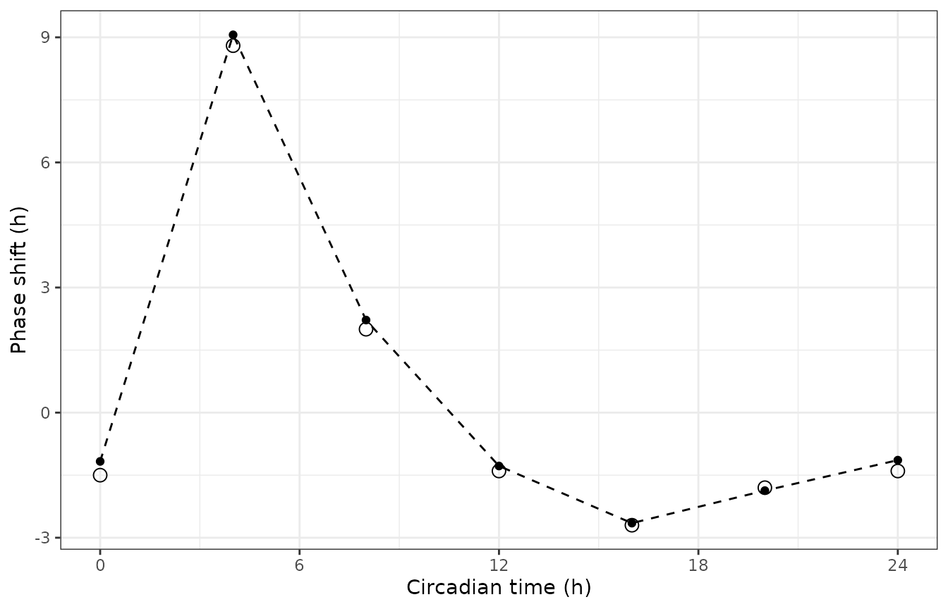
Replicates Figure 3 of Tseng 2025: phase-response curve to 1 h cortisol pulses. Line and filled points = model; open circles = Figure 3.
prc |>
  dplyr::mutate(sim_shift = round(sim_shift, 2), diff = round(sim_shift - paper_shift, 2)) |>
  dplyr::rename(
    "Pulse CT (h)" = ct, "Figure 3 shift (h)" = paper_shift,
    "Simulated shift (h)" = sim_shift, "Difference (h)" = diff
  ) |>
knitr::kable(caption = "Cortisol phase shifts against Figure 3.")| Pulse CT (h) | Figure 3 shift (h) | Simulated shift (h) | Difference (h) |
|---|---|---|---|
| 0 | -1.5 | -1.17 | 0.33 |
| 4 | 8.8 | 9.06 | 0.26 |
| 8 | 2.0 | 2.22 | 0.22 |
| 12 | -1.4 | -1.28 | 0.12 |
| 16 | -2.7 | -2.65 | 0.05 |
| 20 | -1.8 | -1.87 | -0.07 |
| 24 | -1.4 | -1.14 | 0.26 |
The largest advance follows a pulse in the early subjective morning (CT 4), as the paper reports.
Infection without treatment (Figure 5a)
sim_inf <- solve_events(mod, rbind(inoculate(), obs_grid()))
inf_long <- sim_inf |>
  dplyr::select(
    time, `SARS-CoV-2` = total_virus, `Per and Cry mRNAs` = pc_mrna,
    ACE2 = ace2, ISG = isg, cb_RNA = cb_mrna, rev_RNA = rev_mrna
  ) |>
  tidyr::pivot_longer(-time, names_to = "species", values_to = "level")
ggplot(inf_long, aes(time, level, colour = species)) +
  geom_line(linewidth = 0.7) +
  labs(x = "Time (h)", y = "Relative level (a.u.)", colour = NULL) +
  coord_cartesian(ylim = c(0, 2)) +
  theme_bw()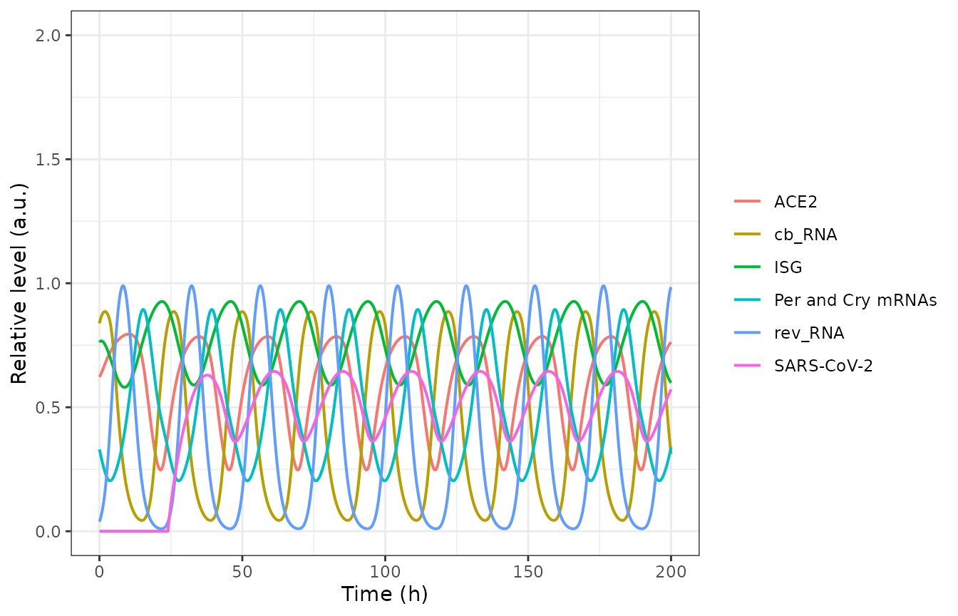
Replicates Figure 5a of Tseng 2025: infection starting at 24 h, no SR9009.
The clock, ACE2 and ISG traces reproduce Figure 5a (for example
pc_RNA peaks of 0.89 every 24 h, ACE2 between about 0.4 and
0.8, ISG between about 0.6 and 0.9). The viral load oscillates with a 24
h period and its peaks fall within about 1.5 h of the figure’s, but it
is lower and its trough comes about 3.5 h earlier than in the
figure:
vir_pk <- peaks(sim_inf$time, sim_inf$total_virus)
vir_tr <- troughs(sim_inf$time, sim_inf$total_virus)
virus_check <- tibble::tibble(
  feature = c("first peak", "first trough"),
  # Figure 5a / Figure S8 'SARS-CoV-2', read by the maintainers.
  paper_time = c(39, 51),
  paper_level = c(1.55, 0.93),
  sim_time = c(vir_pk$time[1], vir_tr$time[1]),
  sim_level = c(vir_pk$value[1], vir_tr$value[1])
)
virus_check |>
  dplyr::mutate(ratio = round(paper_level / sim_level, 2), sim_level = round(sim_level, 3)) |>
  dplyr::rename(
    "Feature" = feature, "Figure time (h)" = paper_time,
    "Figure level (a.u.)" = paper_level, "Model time (h)" = sim_time,
    "Model level (a.u.)" = sim_level, "Figure / model" = ratio
  ) |>
knitr::kable(caption = "Viral load after inoculation at 24 h against Figure 5a.")| Feature | Figure time (h) | Figure level (a.u.) | Model time (h) | Model level (a.u.) | Figure / model |
|---|---|---|---|---|---|
| first peak | 39 | 1.55 | 37.7 | 0.629 | 2.46 |
| first trough | 51 | 0.93 | 47.5 | 0.361 | 2.57 |
stopifnot(
  abs(virus_check$sim_time[1] - virus_check$paper_time[1]) < 2,
  all(abs(diff(vir_pk$time[2:5]) - 24) < 0.5)
)
The published viral load is about 2.4-fold higher than the deposited parameters give; see Assumptions and deviations.
The deposited SBML reading: free virus consumed by entry
In File S1 the free virus is an ordinary reactant of the entry reaction, so a standard SBML simulator depletes it after the single inoculation event. That reading gives a transient infection that is gone within two days, which is not what Figure 5a shows:
mod_sbml <- mod |> rxode2::model(d / dt(vfree) <- -virus_entry)
sim_sbml <- solve_events(mod_sbml, rbind(inoculate(), obs_grid()))
sim_sbml |>
  dplyr::filter(time %in% c(30, 40, 50, 75, 100)) |>
  dplyr::select(time, vfree, total_virus) |>
  dplyr::mutate(dplyr::across(-time, ~ signif(.x, 3))) |>
  dplyr::rename("Time (h)" = time, "Free virus" = vfree, "Total virus" = total_virus) |>
knitr::kable(caption = "Free virus depleted by entry (SBML reaction semantics).")| Time (h) | Free virus | Total virus |
|---|---|---|
| 30 | 2.43e-01 | 1.94e-01 |
| 40 | 1.83e-02 | 5.04e-02 |
| 50 | 3.06e-03 | 5.92e-03 |
| 75 | 1.13e-05 | 3.57e-05 |
| 100 | 0.00e+00 | 2.00e-07 |
stopifnot(sim_sbml$total_virus[sim_sbml$time == 100] < 1e-4)SR9009 at CT 18 (Figure 5b)
SR9009 is switched on for 1 h once a day for five days, starting at CT 18 of the day after inoculation (66 h).
sr_on <- 66 + 24 * (0:4)
sim_sr <- solve_events(mod, rbind(inoculate(), pulse("sr9009", sr_on), obs_grid(by = 0.05)))
sr_long <- sim_sr |>
  dplyr::mutate(Ka_rev_SR9009 = mod$theta[["ka_rev_sr9009"]] * sr9009) |>
  dplyr::select(
    time, `SARS-CoV-2` = total_virus, `Per and Cry mRNAs` = pc_mrna,
    ACE2 = ace2, ISG = isg, cb_RNA = cb_mrna, rev_RNA = rev_mrna, Ka_rev_SR9009
  ) |>
  tidyr::pivot_longer(-time, names_to = "species", values_to = "level")
ggplot(sr_long, aes(time, level, colour = species)) +
  geom_line(linewidth = 0.7) +
  labs(x = "Time (h)", y = "Relative level (a.u.)", colour = NULL) +
  coord_cartesian(ylim = c(0, 2)) +
  theme_bw()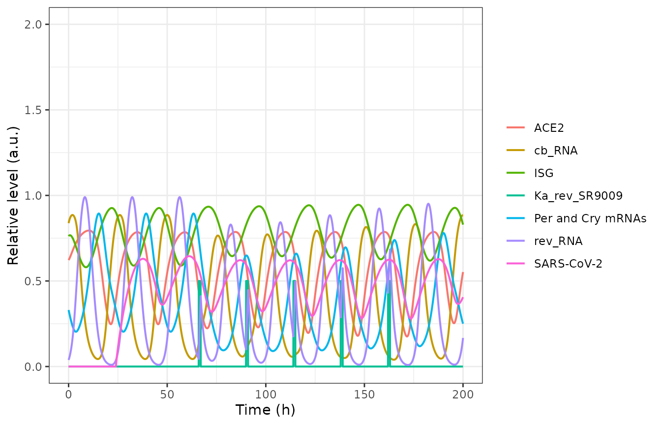
Replicates Figure 5b of Tseng 2025: SR9009 once daily for 1 h starting at CT 18 (66 h).
Figure S8 plots pc_RNA for the same schedule. The SR9009
pulses delay the clock and deepen the pc_RNA trough, and
the peaks recover over the five days; the model reproduces the figure’s
peaks:
pc_sr <- peaks(sim_sr$time, sim_sr$pc_mrna)
pc_sr <- pc_sr[pc_sr$time > 80, ]
s8 <- tibble::tibble(
  cycle = 1:5,
  # Figure S8 'pc_RNA (CT 18)' peaks, read by the maintainers.
  paper_time = c(90, 115, 140, 165, 190),
  paper_peak = c(0.65, 0.66, 0.70, 0.74, 0.78),
  sim_time = pc_sr$time[1:5],
  sim_peak = pc_sr$value[1:5]
)
s8 |>
  dplyr::mutate(sim_peak = round(sim_peak, 3)) |>
  dplyr::rename(
    "Cycle" = cycle, "Figure S8 time (h)" = paper_time,
    "Figure S8 peak" = paper_peak, "Model time (h)" = sim_time,
    "Model peak" = sim_peak
  ) |>
knitr::kable(caption = "pc_RNA peaks under SR9009 at CT 18 against Figure S8.")| Cycle | Figure S8 time (h) | Figure S8 peak | Model time (h) | Model peak |
|---|---|---|---|---|
| 1 | 90 | 0.65 | 90.15 | 0.649 |
| 2 | 115 | 0.66 | 115.35 | 0.660 |
| 3 | 140 | 0.70 | 140.40 | 0.696 |
| 4 | 165 | 0.74 | 165.25 | 0.739 |
| 5 | 190 | 0.78 | 190.10 | 0.780 |
Dosing time (Figure S8)
The paper repeats the five-day course at circadian times 0-24 in 2 h steps and reports CT 18 as the time with the strongest viral repression. With the deposited parameters the viral load at the end of the simulation (200 h) is also lowest after CT 18 dosing:
ct_grid <- seq(0, 24, by = 2)
sweep <- dplyr::bind_rows(lapply(ct_grid, function(ct) {
  s <- solve_events(mod, rbind(inoculate(), pulse("sr9009", 48 + ct + 24 * (0:4)), obs_grid()))
  tibble::tibble(ct = ct, time = s$time, total_virus = s$total_virus, pc_mrna = s$pc_mrna)
}))
sweep_end <- sweep |>
  dplyr::filter(time == 200) |>
  dplyr::select(ct, total_virus)
sweep_end |>
  dplyr::mutate(total_virus = round(total_virus, 3)) |>
  dplyr::rename("Dosing CT (h)" = ct, "Total virus at 200 h (a.u.)" = total_virus) |>
knitr::kable(caption = "Viral load at 200 h after a five-day SR9009 course started at each circadian time.")| Dosing CT (h) | Total virus at 200 h (a.u.) |
|---|---|
| 0 | 0.642 |
| 2 | 0.622 |
| 4 | 0.584 |
| 6 | 0.547 |
| 8 | 0.523 |
| 10 | 0.499 |
| 12 | 0.471 |
| 14 | 0.442 |
| 16 | 0.415 |
| 18 | 0.405 |
| 20 | 0.620 |
| 22 | 0.638 |
| 24 | 0.639 |
sweep |>
  dplyr::mutate(highlight = ct == 18) |>
  tidyr::pivot_longer(c(total_virus, pc_mrna), names_to = "output", values_to = "level") |>
  ggplot(aes(time, level, group = interaction(ct, output), colour = output, alpha = highlight)) +
  geom_line() +
  scale_alpha_manual(values = c(`FALSE` = 0.25, `TRUE` = 1), guide = "none") +
  labs(x = "Time (h)", y = "Relative level (a.u.)", colour = NULL) +
  theme_bw()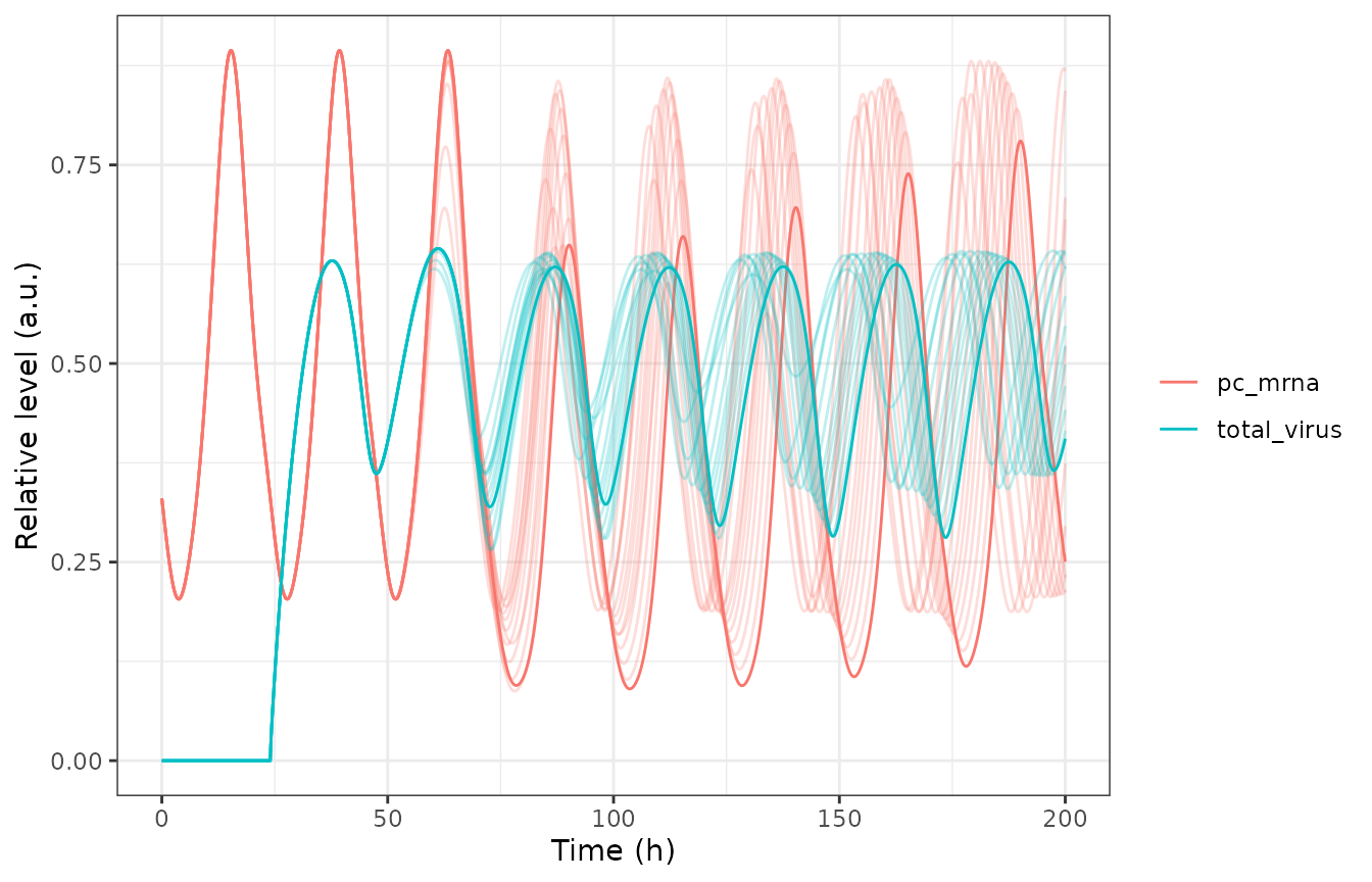
Replicates Figure S8 of Tseng 2025: total virus and pc_RNA for SR9009 courses started at CT 0-24; CT 18 highlighted.
The drug’s antiviral effect is much smaller in the model than in the paper: the viral load at 200 h after CT 18 dosing is 29% below the untreated value, whereas Figure S8 shows the CT 18 curve falling to roughly a fifth of its pre-treatment peaks over the five days.
PKNCA
Not applicable: the model has no drug concentration. SR9009 is represented only by the level of a switched transcription term, and the outputs are relative mRNA, protein and virus levels in arbitrary units. The clock is instead checked against its period, phases, response coefficients and phase-response curve above.
Assumptions and deviations
-
Free virus is not consumed by entry. Data S1 adds
four ODEs for the infection (ACE2, endosomal virus, replicated virus,
ISG) and uses
[Vfree]only as a driver of entry, and Figure 5a shows a sustained, rhythmic infection. The SBML File S1, simulated with standard reaction semantics, instead consumes free virus, which clears the infection within two days. The packaged model follows the printed equations; the SBML reading is shown above withrxode2::model(). -
Viral load is lower than published, and SR9009 suppresses it
less. With the Table S1 / File S1 parameters the viral load
peaks at about 0.63 a.u. instead of the 1.55 a.u. of Figure 5a (peaks
within about 1.5 h of the figure’s, same 24 h rhythm), and the five-day
CT 18 course lowers it by about 30% rather than the roughly five-fold
fall of Figure S8. The clock under SR9009 matches Figure S8 closely, so
the difference lies in the virus layer. Neither reading of the free
virus reproduces the published viral level, and the parameters have not
been adjusted to match the figure. The paper’s viral-load response
coefficients (for example
kd_Vendo= -2.629) are not reproduced either. The deposited sensitivity script never resets the model between its simulations, so each perturbed run starts from the end state of the previous one; that changes a transient output such as the peak viral load, but not the period and amplitude of a limit cycle, and those coefficients are reproduced exactly. -
SR9009 schedule and size. The Methods describe a 4
h exposure started at CT 0 with
Ka_rev_SR9009raised from 0 to 1. The Results, Figure 5b (pulses of 0.5 on the right axis) and File S1 (Ka_rev_SR9009_on= 0.5,SP= 1 h) agree on a 1 h exposure of 0.5, and that is what reproduces Figure S8; the packaged value is 0.5 and the vignette gives 1 h doses. -
SR9009 has no pharmacokinetics. The dose is the
on/off level of the
Ka_rev_SR9009term, as in the paper. A dose level other than 1 scales the term linearly, which the paper did not explore. -
Unused SBML elements omitted. File S1 also contains
a KL001 arm whose on and off values are identical
(
Krep_dPC_KL0011 -> 1,Ki_ACE2_PCC2.4 -> 2.4), dummy gene species consumed by transcription that no rate depends on, and bookkeeping events that record the period and amplitude. None of these changes any trajectory and none is in the paper, so they are not part of the packaged model. -
Labels in Table S1. Table S1 lists
Ka_ACE2_CBandKa_ISG_PCand labelsk_ISG‘Virus production rate’; the SBML file and Data S1 show these are the CLOCK:BMAL1 threshold on ACE2, the PER:CRY threshold on ISG, and the ISG production rate. Data S1 Eq. 5 printsH_rev_CBforH_rev_CBC. -
Fixed parameters. Only the five mRNA degradation
rates, which the Methods say were taken from experimental data or
published models, and the two constant boundary levels
(
ace2_mrna,isg_pre) are markedfixed(). Every other value was tuned by hand rather than estimated; no parameter carries an uncertainty. -
Digitised targets. The Figure 2b windows, the
Figure 3 phase shifts, the Figure 5a viral levels and the Figure S8
pc_RNApeaks were read from the figures by the maintainers. - No correction notice for the article was found on PubMed or the publisher’s page as of 2026-11-02.