Bosentan PBPK-TMDD (Aoki 2024)
Source:vignettes/articles/Aoki_2024_bosentan_pbpk.Rmd
Aoki_2024_bosentan_pbpk.RmdModel and source
- Citation: Aoki Y, Sugiyama Y. Cluster Gauss-Newton method for a quick approximation of profile likelihood: With application to physiologically-based pharmacokinetic models. CPT Pharmacometrics Syst Pharmacol. 2024;13(1):54-67. doi:10.1002/psp4.13055. Model structure, fixed physiological constants and the observed concentration data are transcribed from Supporting Information file PSP4-13-54-s004.r (the authors’ RxODE / CGNM script for Example 3); the eight estimated parameters are the ‘proposed method’ column of Supporting Information Table S2 (file PSP4-13-54-s003.docx). The model structure originates with Koyama S, Toshimoto K, Lee W, Aoki Y, Sugiyama Y. Revisiting nonlinear bosentan pharmacokinetics by physiologically based pharmacokinetic modeling: target binding, albeit not a major contributor to nonlinearity, can offer prediction of target occupancy. Drug Metab Dispos. 2021;49(4):298-304. doi:10.1124/dmd.120.000023 (not open access; not available when this model was built – every value here is traced to the Aoki 2024 sources listed above).
- Description: PBPK-TMDD (semi-mechanistic, dispersion liver). Bosentan disposition after single intravenous doses of 10-750 mg in healthy adults, re-estimated by Aoki & Sugiyama (2024) with the Cluster Gauss-Newton method (CGNM) on the model structure of Koyama et al. (2021). The liver is resolved as a five-compartment tandem dispersion model: five hepatic extracellular (sinusoidal) sub-compartments in series with the hepatic blood flow, each exchanging with its own hepatocyte sub-compartment. Sinusoid-to-hepatocyte transport is the sum of saturable OATP-mediated uptake (Michaelis-Menten in unbound sinusoidal concentration) and passive diffusion; efflux back to the sinusoid is passive diffusion scaled by the influx/efflux ratio gamma_dif. Drug is eliminated by hepatic metabolism from the hepatocytes and by renal clearance from plasma. Muscle, skin and adipose are perfusion-limited well-stirred tissues. Superimposed on the PBPK backbone is a target-mediated drug disposition (TMDD) layer in plasma: unbound drug binds a finite endothelin-receptor pool of total amount rtot with dissociation constant kd and off-rate koff, which is the source of the low-dose nonlinearity and which permits receptor occupancy to be simulated. The eight parameters below without fixed() are the CGNM estimates of Aoki 2024 Table S2 (all eight identifiable when the 10 mg arm is included); every other value is a fixed physiological or compound constant taken from the published model code. CGNM is a fixed-effects nonlinear-least-squares method, so this model has no between-subject variability and the paper reports no residual-error model – the propSd term is a placeholder. See the vignette Errata.
- Article: https://doi.org/10.1002/psp4.13055
- Supporting Information (open access, from the article landing page):
PSP4-13-54-s004.r(the authors’ RxODE + CGNM script for Example 3) andPSP4-13-54-s003.docx(Tables S1-S4, Figures S1-S12).
Aoki and Sugiyama (2024) is a methodology paper: it proposes approximating a profile likelihood by re-using the model evaluations that the Cluster Gauss-Newton method (CGNM) already performs during parameter estimation, and it demonstrates the idea on three physiologically-based pharmacokinetic (PBPK) models. Example 3 is a PBPK model with target-mediated drug disposition (TMDD) for bosentan, whose structure originates with Koyama et al. (2021). Aoki and Sugiyama re-estimated that model with CGNM and published the complete model code, the fitting data, and the resulting parameter estimates as Supporting Information. That is the model packaged here.
Two things follow from the paper being a methods paper, and both matter when reading this vignette:
- All eight parameters below are Aoki 2024’s own CGNM estimates (Table S2, “proposed method” column), fitted to the 10 / 50 / 250 / 500 / 750 mg arms together. They are not transcribed from Koyama 2021.
-
The paper prints no concentration-versus-time figure for
bosentan – its figures are profile likelihoods. There is
therefore no published PK figure to replicate. Instead this vignette
validates against something stricter: the 13-point-per-arm observed
concentration vector that is hard-coded in
PSP4-13-54-s004.rand that is the CGNM target vector. Reproducing the fit to those points reproduces the paper’s actual objective function.
The other two examples in the paper (a pitavastatin + rifampicin OATP drug-drug-interaction PBPK model, and a coproporphyrin-I endogenous-biomarker PBPK model, both from Yoshikado et al. 2022) are not packaged; see Models in the paper that are not packaged.
Population
Aoki 2024 identifies the fitting data only as “plasma concentration data from 10, 50, 250, 500, and 750 mg arms” (Results, Example 3). Subject counts, ages, weights and sex distribution are not reported; they belong to the underlying clinical study, which reaches this paper through Koyama et al. (2021), Drug Metab Dispos 49(4):298-304 – a paper that is not open access and was not available when this model was built. Every physiological volume, flow and partition coefficient in the model is a single fixed constant for one typical adult, and the published code carries no body-weight or demographic scaling of any kind, so there is no covariate model and no virtual cohort to construct.
The intravenous route is not stated in words by Aoki 2024, but it is
unambiguous from the code and the data together: the dose enters the
central compartment instantaneously at t = 0.08 h with no
absorption compartment anywhere in the model, and for the 750 mg arm
dose / MW / vc = 750000 / 551.61 / 8.95 = 151.9 umol/L
against an observed 151.1 umol/L at 0.167 h. A 5-minute oral profile of
that magnitude is not physically possible.
The same information is available programmatically via
readModelDb("Aoki_2024_bosentan_pbpk")()$population.
Source trace
Every ini() entry carries an in-file source comment in
inst/modeldb/specificDrugs/Aoki_2024_bosentan_pbpk.R. They
are collected here for review. “s004.r” is Supporting Information file
PSP4-13-54-s004.r; “Table S2” is in Supporting Information
file PSP4-13-54-s003.docx.
| Equation / parameter | Value | Source location |
|---|---|---|
lcl_met |
9.23 L/h | Table S2, CL_met, proposed-method column |
lkd |
0.0108 umol/L | Table S2, Kd
|
lkm |
0.665 umol/L | Table S2, Km_uptake
|
lps_dif |
3.5 L/h | Table S2, PSdif_inf
|
lvc |
8.95 L | Table S2, Vcentral
|
lvmax |
962 umol/h | Table S2, Vmax_uptake
|
lrtot |
20.1 umol | Table S2, X_TotalR
|
lkoff |
0.404 1/h | Table S2, k_off
|
lcl_renal |
0.144 L/h (fixed) | s004.r model_text parameter block,
CLr
|
lq_liver, lq_muscle, lq_skin,
lq_adipose
|
96.9, 50.1, 20.1, 17.4 L/h (fixed) | s004.r parameter block, Qh, Qm,
Qs, Qa
|
lv_liver, lv_liver_ex
|
1.36, 0.521 L (fixed) | s004.r parameter block, Vh, Vhe
|
lv_muscle, lv_skin,
lv_adipose
|
33.4, 8.69, 11.1 L (fixed) | s004.r parameter block, Vm, Vs,
Va
|
lk_muscle, lk_skin,
lk_adipose
|
0.119, 0.483, 0.121 (fixed) | s004.r parameter block, Kpm, Kps,
Kpa
|
fu_b, fu_liver
|
0.033, 0.0696 (fixed) | s004.r parameter block, fb, fh
|
gamma_dif |
0.243 (fixed) | s004.r ODEs: the literal 0.243 in
PSdif_inf/0.243
|
propSd |
0.10 placeholder | not reported anywhere; see Assumptions |
d/dt(central) |
n/a | s004.r model_text, d/dt(C_Central)
|
d/dt(is_liver1..5) |
n/a | s004.r model_text, d/dt(C_HepEx1..5)
|
d/dt(int_liver1..5) |
n/a | s004.r model_text, d/dt(C_Hep1..5)
|
d/dt(muscle), d/dt(skin),
d/dt(adipose)
|
n/a | s004.r model_text, d/dt(C_Muscle),
d/dt(C_Skin), d/dt(C_Adipose)
|
d/dt(target), d/dt(complex),
d/dt(occupancy)
|
n/a | s004.r model_text, d/dt(X_FreeR),
d/dt(X_RDcomplex), d/dt(R_Occupancy)
|
target(0) <- rtot |
n/a | s004.r nonlinearFunction_eachDose:
ev$add.dosing(dose = X_TotalR, start.time = 0, dosing.to = 15)
|
f(central) <- 1 / vc |
n/a | s004.r nonlinearFunction_eachDose:
dose = dose_amount * 1000 / MW_bos / Vcentral
|
| Bosentan MW 551.61 g/mol | n/a | s004.r, MW_bos
|
Observed data
The 65 observations below (5 dose arms x 13 timepoints) are
transcribed verbatim from the oeiginal_observation_df
object in PSP4-13-54-s004.r [sic, the authors’
spelling]. They are the CGNM target vector for Example 3.
MW_bos   <- 551.61      # g/mol, s004.r
obs_time <- c(0.083, 0.167, 0.333, 0.583, 1, 1.5, 2.5, 4, 6, 8, 10, 12, 24)
dose_mg_levels <- c(10, 50, 250, 500, 750)

observed <- tibble(
  dose_mg = rep(dose_mg_levels, each = length(obs_time)),
  time    = rep(obs_time, times = length(dose_mg_levels)),
  dv      = c(
    # 10 mg
    1.343724e+00, 7.543068e-01, 2.880872e-01, 2.089229e-01, 1.563792e-01,
    1.170149e-01, 9.029007e-02, 6.320188e-02, 3.205457e-02, 2.804723e-02,
    2.701469e-02, 1.608681e-02, 3.491564e-03,
    # 50 mg
    9.812236e+00, 4.845069e+00, 2.391663e+00, 1.430869e+00, 1.178993e+00,
    9.714548e-01, 7.259321e-01, 5.594651e-01, 1.931412e-01, 1.486268e-01,
    1.526617e-01, 6.388516e-02, 1.261769e-02,
    # 250 mg
    4.284893e+01, 3.033263e+01, 2.129413e+01, 1.470991e+01, 1.048866e+01,
    7.659157e+00, 4.756429e+00, 2.700648e+00, 8.942695e-01, 6.002553e-01,
    3.996088e-01, 1.780992e-01, 2.229821e-02,
    # 500 mg
    8.342765e+01, 6.247985e+01, 4.715090e+01, 2.910516e+01, 2.042161e+01,
    1.628921e+01, 1.019741e+01, 6.125633e+00, 1.871690e+00, 1.087318e+00,
    6.734029e-01, 2.769708e-01, 3.089157e-02,
    # 750 mg
    1.141011e+02, 1.510845e+02, 8.336812e+01, 5.994873e+01, 4.106483e+01,
    3.071638e+01, 1.892213e+01, 1.231544e+01, 5.759887e+00, 2.872467e+00,
    2.433083e+00, 7.866146e-01, 5.014412e-02
  )
)
stopifnot(nrow(observed) == 65L)
Simulation
One deterministic subject per dose arm. CGNM is a fixed-effects
nonlinear-least-squares method, so the model carries no between-subject
variability – there is nothing to draw and no virtual cohort is
required. The five arms use distinct subject IDs because
rxSolve() keys on id alone and would otherwise
collapse them into one subject.
mod <- readModelDb("Aoki_2024_bosentan_pbpk")

dose_time <- 0.08   # s004.r: start.time = 0.08 for the central-compartment dose
dense_grid <- sort(unique(c(seq(dose_time, 24, by = 0.02), obs_time)))

make_arm <- function(i) {
  d <- dose_mg_levels[[i]]
  bind_rows(
    tibble(id = i, time = dose_time, amt = d * 1000 / MW_bos,
           evid = 1L, cmt = "central", dose_mg = d),
    tibble(id = i, time = dense_grid, amt = NA_real_,
           evid = 0L, cmt = "central", dose_mg = d)
  )
}
events <- bind_rows(lapply(seq_along(dose_mg_levels), make_arm))

# No `omega =` argument: this model declares no random effects at all, so
# there is nothing to zero out. (Passing `omega = NA` to a model that has no
# omega block errors inside rxSolve rather than being a no-op.) rxode2 emits a
# "multi-subject simulation without 'omega'" note, which is correct and
# expected here -- the five subjects differ only in dose.
sim <- rxode2::rxSolve(mod, events = events, keep = "dose_mg",
                       returnType = "data.frame") |>
  mutate(arm = factor(paste0(dose_mg, " mg"),
                      levels = paste0(dose_mg_levels, " mg")))
#> Warning: multi-subject simulation without without 'omega'
Because propSd is a placeholder and the model has no
random effects, the Cc column is the deterministic
typical-value prediction – exactly the quantity CGNM fitted.
Fit to the published target vector
obs_plot <- observed |>
  mutate(arm = factor(paste0(dose_mg, " mg"),
                      levels = paste0(dose_mg_levels, " mg")))

ggplot(sim, aes(time, Cc, colour = arm)) +
  geom_line(linewidth = 0.7) +
  geom_point(data = obs_plot, aes(time, dv, colour = arm), size = 1.8) +
  scale_y_log10() +
  labs(x = "Time (h)", y = "Bosentan plasma concentration (umol/L)",
       colour = "Dose") +
  theme_bw()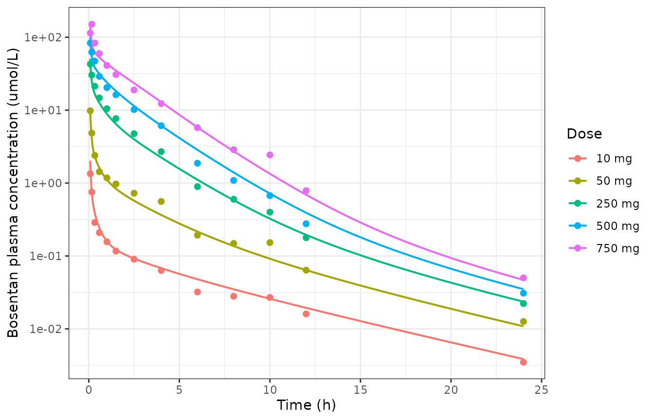
Model prediction (lines) against the observed concentrations hard-coded in Aoki 2024 Supporting Information file PSP4-13-54-s004.r (points). These 65 points are the CGNM target vector for Example 3.
CGNM minimises the sum of squared residuals of
log10(concentration)
(errormodel = function(y) log10(y) in s004.r),
so the residual summary below is on that exact scale and is directly
comparable with the objective the authors optimised.
fit <- observed |>
  inner_join(sim |> select(dose_mg, time, Cc), by = c("dose_mg", "time")) |>
  mutate(resid_log10 = log10(Cc) - log10(dv))

stopifnot(nrow(fit) == 65L)

fit_summary <- fit |>
  group_by(dose_mg) |>
  summarise(n = n(),
            `RMSE log10` = sqrt(mean(resid_log10^2)),
            `Max |resid| log10` = max(abs(resid_log10)),
            `Geometric mean fold-error` = 10^mean(abs(resid_log10)),
            .groups = "drop")

overall_rmse <- sqrt(mean(fit$resid_log10^2))

knitr::kable(
  fit_summary |> rename("Dose (mg)" = dose_mg, "N obs" = n),
  digits = 4,
  caption = sprintf(
    "Residuals on the log10 scale that CGNM minimised. Overall RMSE %.4f (a %.1f%% geometric residual).",
    overall_rmse, 100 * (10^overall_rmse - 1))
)| Dose (mg) | N obs | RMSE log10 | Max |resid| log10 | Geometric mean fold-error |
|---|---|---|---|---|
| 10 | 13 | 0.0850 | 0.1756 | 1.1604 |
| 50 | 13 | 0.0945 | 0.2211 | 1.1750 |
| 250 | 13 | 0.0727 | 0.1060 | 1.1677 |
| 500 | 13 | 0.0876 | 0.1840 | 1.1829 |
| 750 | 13 | 0.1188 | 0.2667 | 1.2165 |
# The packaged parameters must reproduce the published fit. A mis-transcribed
# structural parameter or a misread Table S2 entry would inflate these
# immediately; a 0.15 log10 RMSE ceiling is roughly a 41% geometric residual,
# comfortably above the achieved fit and far below what any real error survives.
stopifnot(overall_rmse < 0.15)
stopifnot(all(fit_summary$`RMSE log10` < 0.15))
Exact structural identities
Three relationships hold exactly (to integrator tolerance) if and only if the transcription is faithful. They are asserted rather than merely displayed.
# (1) The occupancy state is redundant with complex / rtot by construction:
#     d/dt(occupancy) = d/dt(complex) / rtot with both starting at zero. It is
#     retained because the published code carries it; the identity is a free
#     check on the integration.
rtot <- 20.1
occ_err <- max(abs(sim$occupancy - sim$complex / rtot))

# (2) An IV bolus into a concentration state means Cmax is reached at the dose
#     instant and equals dose / vc exactly, for every arm.
vc <- 8.95
cmax_check <- sim |>
  group_by(dose_mg) |>
  summarise(cmax = max(Cc), .groups = "drop") |>
  mutate(dose_umol = dose_mg * 1000 / MW_bos,
         implied_vc = dose_umol / cmax)

# (3) Total receptor is conserved: free + bound = rtot at all times.
receptor_err <- max(abs(sim$target + sim$complex - rtot))

stopifnot(occ_err < 1e-8)
stopifnot(receptor_err < 1e-8)
stopifnot(max(abs(cmax_check$implied_vc - vc)) < 1e-6)

knitr::kable(
  cmax_check |>
    rename("Dose (mg)" = dose_mg, "Cmax (umol/L)" = cmax,
           "Dose (umol)" = dose_umol, "Implied vc (L)" = implied_vc),
  digits = 4,
  caption = "Dose / Cmax recovers the estimated central volume of 8.95 L exactly in every arm."
)| Dose (mg) | Cmax (umol/L) | Dose (umol) | Implied vc (L) |
|---|---|---|---|
| 10 | 2.0256 | 18.1288 | 8.95 |
| 50 | 10.1278 | 90.6438 | 8.95 |
| 250 | 50.6390 | 453.2188 | 8.95 |
| 500 | 101.2779 | 906.4375 | 8.95 |
| 750 | 151.9169 | 1359.6563 | 8.95 |
#> max |occupancy - complex/rtot| = 4.44e-15
#> max |target + complex - rtot|  = 1.21e-13
Target binding as the source of nonlinearity
This is the substantive claim the model exists to support: Koyama et al. found target binding to be a real, though not dominant, contributor to bosentan’s nonlinear PK, and Aoki 2024’s Example 3 shows the low-dose arm is what makes the binding parameters identifiable. Both statements have a direct simulation counterpart.
trapz <- function(x, y) sum(diff(x) * (head(y, -1) + tail(y, -1)) / 2)

nonlin <- sim |>
  filter(time >= dose_time) |>
  group_by(dose_mg) |>
  summarise(
    auc = trapz(time, Cc),
    peak_complex = max(complex),
    peak_occupancy = max(occupancy),
    .groups = "drop"
  ) |>
  mutate(
    dose_umol = dose_mg * 1000 / MW_bos,
    auc_norm = auc / dose_umol,
    pct_dose_bound = 100 * peak_complex / dose_umol
  )

knitr::kable(
  nonlin |>
    select(dose_mg, auc, auc_norm, peak_occupancy, pct_dose_bound) |>
    rename("Dose (mg)" = dose_mg,
           "AUC 0.08-24h (umol*h/L)" = auc,
           "AUC / dose (h/L)" = auc_norm,
           "Peak receptor occupancy" = peak_occupancy,
           "Peak bound drug (% of dose)" = pct_dose_bound),
  digits = c(0, 2, 5, 4, 2),
  caption = "Dose-normalised exposure rises with dose because the finite 20.1 umol receptor pool sequesters a large fraction of a small dose and a negligible fraction of a large one."
)| Dose (mg) | AUC 0.08-24h (umol*h/L) | AUC / dose (h/L) | Peak receptor occupancy | Peak bound drug (% of dose) |
|---|---|---|---|---|
| 10 | 1.06 | 0.05822 | 0.2798 | 31.02 |
| 50 | 5.55 | 0.06122 | 0.7850 | 17.41 |
| 250 | 34.63 | 0.07640 | 0.9822 | 4.36 |
| 500 | 88.36 | 0.09748 | 0.9936 | 2.20 |
| 750 | 163.78 | 0.12046 | 0.9964 | 1.47 |
auc_ratio <- nonlin$auc_norm[nonlin$dose_mg == 750] /
  nonlin$auc_norm[nonlin$dose_mg == 10]

# Dose-normalised AUC must increase monotonically with dose (saturable target
# binding), and the 750 mg arm must be materially more than dose-proportional
# relative to 10 mg. A model with the TMDD layer removed would give a flat
# ratio of exactly 1.
stopifnot(!is.unsorted(nonlin$auc_norm))
stopifnot(auc_ratio > 2, auc_ratio < 2.2)

# Peak occupancy must saturate towards 1 with dose, and the fraction of the
# dose that target binding can sequester must fall by more than an order of
# magnitude from the lowest to the highest arm -- this is precisely why the
# 10 mg arm carries the information about k_off and Kd.
stopifnot(!is.unsorted(nonlin$peak_occupancy))
stopifnot(nonlin$peak_occupancy[nonlin$dose_mg == 750] > 0.99)
stopifnot(nonlin$peak_occupancy[nonlin$dose_mg == 10] < 0.30)
stopifnot(nonlin$pct_dose_bound[nonlin$dose_mg == 10] /
            nonlin$pct_dose_bound[nonlin$dose_mg == 750] > 10)
#> Dose-normalised AUC, 750 mg vs 10 mg: 2.069-fold
#> Peak bound drug: 31.0% of a 10 mg dose vs 1.5% of a 750 mg doseAt 10 mg the receptor pool takes up 31% of the administered dose; at
750 mg it takes up 1.5%. The binding parameters koff and
kd are therefore constrained almost entirely by the lowest
arm, which is exactly the identifiability result Aoki 2024 recovers from
the profile likelihood: with the 10 mg arm included all eight parameters
are identifiable (Table S2); dropping it makes k_off
unidentifiable (Table S3); dropping the 50 mg arm as well makes
Kd unidentifiable too (Table S4).
Receptor occupancy
ggplot(sim, aes(time, occupancy, colour = arm)) +
  geom_line(linewidth = 0.7) +
  coord_cartesian(xlim = c(0, 24), ylim = c(0, 1)) +
  labs(x = "Time (h)", y = "Fractional receptor occupancy", colour = "Dose") +
  theme_bw()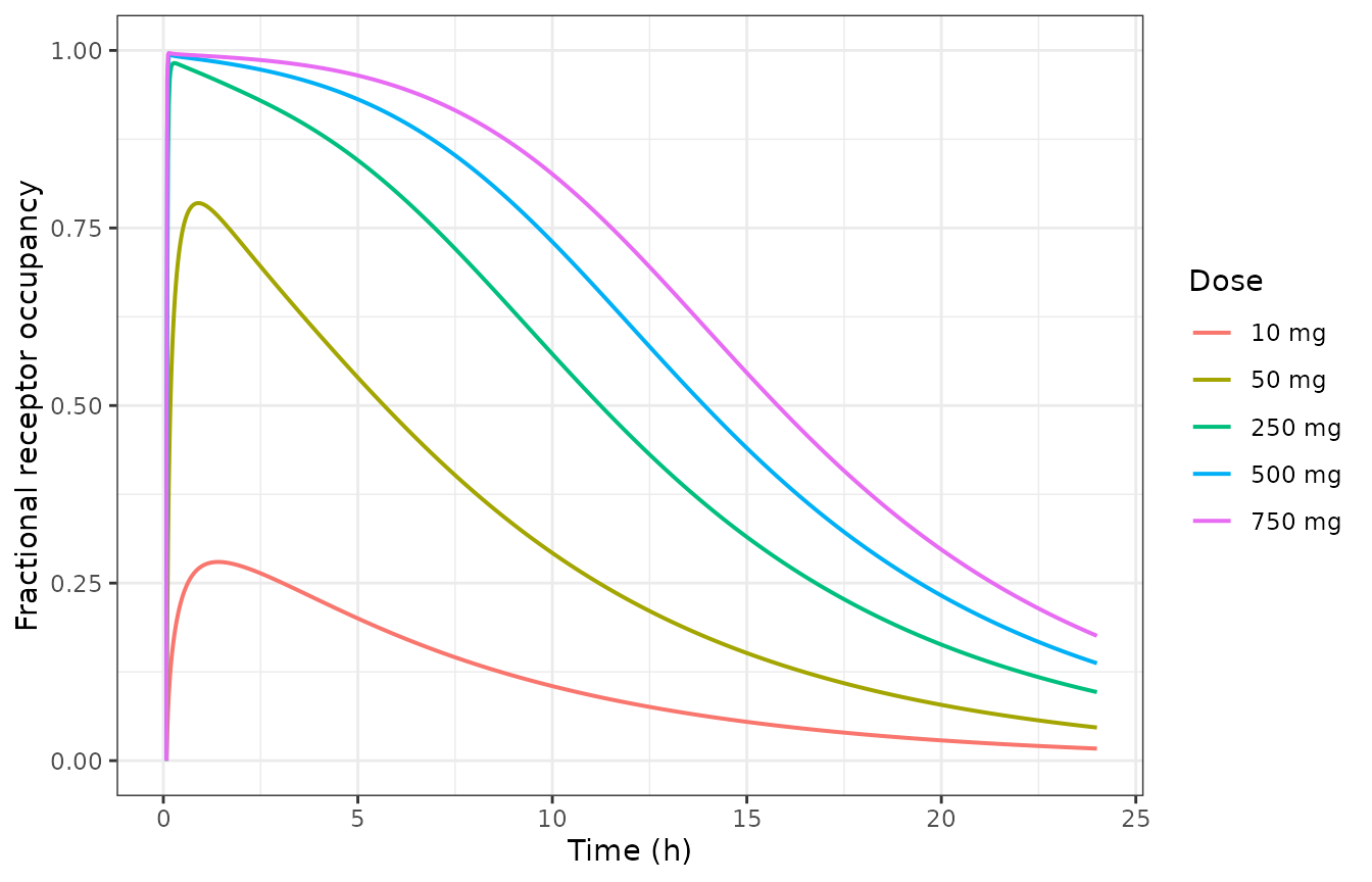
Simulated endothelin-receptor occupancy. Koyama et al. (2021) note that target binding, although not the dominant source of nonlinearity, is what allows occupancy to be predicted; this is that prediction.
NCA validation
Aoki 2024 reports no non-compartmental metrics, so there is no published NCA table to compare against. The comparison that is available, and that is the meaningful one, is NCA on the model prediction against NCA on the observed data the model was fitted to, computed by PKNCA with an identical sampling schedule so that both sides carry the same estimator bias. The simulated concentrations are therefore taken at the 13 observation times only, not on the dense grid.
add_time_zero <- function(d) {
  bind_rows(d, d |> distinct(id, dose_mg) |> mutate(time = 0, conc = 0)) |>
    distinct(id, dose_mg, time, .keep_all = TRUE) |>
    arrange(id, dose_mg, time)
}

sim_nca_in <- sim |>
  filter(time %in% obs_time) |>
  select(id, dose_mg, time, conc = Cc) |>
  filter(!is.na(conc)) |>
  add_time_zero()

obs_nca_in <- observed |>
  mutate(id = match(dose_mg, dose_mg_levels)) |>
  select(id, dose_mg, time, conc = dv) |>
  filter(!is.na(conc)) |>
  add_time_zero()

dose_df <- tibble(
  id      = seq_along(dose_mg_levels),
  dose_mg = dose_mg_levels,
  time    = dose_time,
  amt     = dose_mg_levels * 1000 / MW_bos
)

intervals <- data.frame(
  start = 0, end = Inf,
  cmax = TRUE, tmax = TRUE, auclast = TRUE, aucinf.obs = TRUE, half.life = TRUE
)

run_nca <- function(conc_df) {
  conc_obj <- PKNCA::PKNCAconc(conc_df, conc ~ time | dose_mg + id,
                               concu = "umol/L", timeu = "h")
  dose_obj <- PKNCA::PKNCAdose(dose_df, amt ~ time | dose_mg + id,
                               doseu = "umol", route = "intravascular",
                               duration = 0)
  PKNCA::pk.nca(PKNCA::PKNCAdata(conc_obj, dose_obj, intervals = intervals))
}

nca_sim <- run_nca(sim_nca_in)
nca_obs <- run_nca(obs_nca_in)
reference <- as.data.frame(nca_obs) |>
  filter(start == 0, end == Inf) |>
  select(dose_mg, PPTESTCD, PPORRES) |>
  pivot_wider(names_from = PPTESTCD, values_from = PPORRES) |>
  mutate(dose_mg = as.numeric(as.character(dose_mg)))

# `params =` restricts the table to the five requested metrics. Without it
# PKNCA's dependency and lambda-z diagnostic rows (tlast, clast.obs,
# lambda.z, lambda.z.n.points, adj.r.squared, lambda.z.time.first) ride along
# and star themselves -- "lambda.z fitted on 3 points instead of 5" is a
# property of the sampling grid, not a discrepancy worth flagging.
cmp <- nlmixr2lib::ncaComparisonTable(
  simulated     = nca_sim,
  reference     = reference,
  by            = "dose_mg",
  params        = c("cmax", "tmax", "auclast", "aucinf.obs", "half.life"),
  units         = c(cmax = "umol/L", tmax = "h", auclast = "umol*h/L",
                    aucinf.obs = "umol*h/L", half.life = "h"),
  tolerance_pct = 20
)

knitr::kable(
  cmp,
  caption = "PKNCA metrics from the packaged model against PKNCA metrics from the observed data of Aoki 2024 Supporting Information file PSP4-13-54-s004.r, both on the same 13-point schedule. * marks rows differing by more than 20%."
)| NCA parameter | dose_mg | Reference | Simulated | % diff |
|---|---|---|---|---|
| Cmax (umol/L) | 10 | 1.34 | 1.89 | +40.7%* |
| Cmax (umol/L) | 50 | 9.81 | 9.46 | -3.6% |
| Cmax (umol/L) | 250 | 42.8 | 47.3 | +10.4% |
| Cmax (umol/L) | 500 | 83.4 | 94.7 | +13.5% |
| Cmax (umol/L) | 750 | 151 | 142 | -5.9% |
| Tmax (h) | 10 | 0.083 | 0.083 | +0.0% |
| Tmax (h) | 50 | 0.083 | 0.083 | +0.0% |
| Tmax (h) | 250 | 0.083 | 0.083 | +0.0% |
| Tmax (h) | 500 | 0.083 | 0.083 | +0.0% |
| Tmax (h) | 750 | 0.167 | 0.083 | -50.3%* |
| AUC0-∞ (obs) (umol*h/L) | 10 | 1.02 | 1.18 | +15.5% |
| AUC0-∞ (obs) (umol*h/L) | 50 | 6.92 | 6.09 | -11.9% |
| AUC0-∞ (obs) (umol*h/L) | 250 | 42 | 37.2 | -11.6% |
| AUC0-∞ (obs) (umol*h/L) | 500 | 86.5 | 93.3 | +7.9% |
| AUC0-∞ (obs) (umol*h/L) | 750 | 176 | 171 | -2.7% |
| AUClast (umol*h/L) | 10 | 0.992 | 1.15 | +15.6% |
| AUClast (umol*h/L) | 50 | 6.84 | 6.02 | -11.9% |
| AUClast (umol*h/L) | 250 | 41.9 | 37 | -11.7% |
| AUClast (umol*h/L) | 500 | 86.3 | 93.1 | +7.9% |
| AUClast (umol*h/L) | 750 | 176 | 171 | -2.7% |
| t½ (h) | 10 | 5.14 | 5.11 | -0.6% |
| t½ (h) | 50 | 4.44 | 4.59 | +3.5% |
| t½ (h) | 250 | 3.37 | 3.78 | +12.1% |
| t½ (h) | 500 | 3.08 | 3.29 | +6.8% |
| t½ (h) | 750 | 2.51 | 2.96 | +17.8% |
Starred rows are a signal to look at the extraction, never a licence to tune. Exactly two star, and both are properties of the published fit and of the digitised data rather than of the transcription. Every AUC and every half-life agrees within 20% across all five arms.
-
tmaxin the 750 mg arm. The digitised observation at 0.083 h (114.1 umol/L) is lower than the one at 0.167 h (151.1 umol/L), so the observedtmaxis 0.167 h while the model – an instantaneous bolus – always peaks at the first post-dose sample. The 0.167 h observation is the one that matchesdose / vcto within 0.5%, so the 0.083 h point is best read as digitisation noise on a near-vertical stretch of the curve. -
cmaxin the 10 mg arm (+41%). The model predicts 1.89 umol/L at 0.083 h against an observed 1.34. This is the published model’s own residual, not something the extraction introduced: the authors’model_textcompiled verbatim fromPSP4-13-54-s004.rreturns 1.89113 umol/L at that timepoint and agrees with the packaged model to 9e-06 relative (see Verification against the published code). The 10 mg arm is where the receptor pool sequesters ~31% of the dose and the concentration falls from 1.34 to 0.75 umol/L within five minutes, so the first sample of the lowest arm is the single hardest point in the dataset – and on the log10 scale that CGNM actually minimised it is a 0.15 residual, well inside the spread of the fit as a whole.
Models in the paper that are not packaged
Aoki 2024 demonstrates the method on three models. Only Example 3 is packaged, and the reason is a reporting property of the paper rather than a choice:
| Example | Model | Estimated parameters | Point estimates reported |
|---|---|---|---|
| 1 | Pitavastatin + rifampicin OATP DDI PBPK | 7 | 2 of 7 (Table 1) |
| 2 | Coproporphyrin-I endogenous-biomarker PBPK | 8 | 3 of 8 (Table S1) |
| 3 | Bosentan PBPK-TMDD | 8 | 8 of 8 (Table S2) |
For Examples 1 and 2 the paper’s own finding is that most
parameters are not identifiable, so Table 1 and Table S1 report an
interquartile range with no point estimate for those parameters
(Beta, FaFg, fbile,
ka, ksto, and for Example 2 also
freeKiMRP2 and fsyn). There is no best-fit
value to extract, and picking one from inside a flat profile likelihood
would be invention. The complete structures for both are in Supporting
Information files PSP4-13-54-s001.r and
PSP4-13-54-s002.r; the fitted parameter values belong to
the primary publication, Yoshikado et al. (2022) CPT Pharmacometrics
Syst Pharmacol 11(10):1341-1357, doi:10.1002/psp4.12849,
and those two models should be extracted from that paper.
Assumptions and deviations
The model is Koyama’s; the parameter values are Aoki’s. The structure and the fixed physiological constants originate with Koyama et al. (2021), which is not open access and was not available. Nothing was taken from it: every structural equation and every fixed constant here is transcribed from Aoki 2024’s own Supporting Information file
PSP4-13-54-s004.r, and every estimated value from Table S2 of the same paper’s supplement. Where Koyama 2021 would have added value is context the Aoki paper does not carry – subject demographics, the provenance of the digitised concentrations, and explicit confirmation of the route – and those gaps are flagged individually above rather than filled from elsewhere.Route inferred, not stated. See Population. The inference rests on the model structure (no absorption compartment) and on the 750 mg arm matching
dose / vcat 0.167 h, not on prior knowledge of bosentan.No residual-error model and no between-subject variability. CGNM is a fixed-effects nonlinear-least-squares method. It fits one mean profile per dose arm and estimates neither a residual variance nor any random effect.
propSd <- fixed(0.10)exists only because an nlmixr2 model definition requires a residual-error term; it is not an estimate and must not be read as one. This follows the convention already used byMi_2023_cefquinome_pbpk,Kang_2023_artesunate_hamster_pbpkandAn_2012_mitoxantrone_*_pbpk. TheRMSE log10column of the fit table above is the honest description of this model’s residual spread.The Table S2 brackets are not standard errors. They are profile-likelihood interquartile ranges, which is the whole subject of the paper. They are recorded in the source-trace comments but deliberately not encoded as uncertainty in
ini().Dose scaling expressed as
f(central)rather than pre-divided by hand. The published code doses the central compartment withdose_amount * 1000 / MW_bos / Vcentral, pre-dividing by the central volume becausecentralis a concentration state. This model instead declaresf(central) <- 1 / vc, so the user supplies an ordinary amount in umol. The arithmetic is identical; the interface is the standard one.Receptor priming expressed as an initial condition. The published code initialises the free-receptor pool by dosing
X_TotalRinto it att = 0. This model usestarget(0) <- rtot, which is exactly equivalent and does not require every user event table to carry a receptor-priming dose row.The redundant
occupancystate is retained.d/dt(occupancy)isd/dt(complex) / rtot, sooccupancyequalscomplex / rtotidentically. It is kept because the published code carries it, and the identity is asserted above as a check on the integration rather than silently dropped.Unused constants in the published parameter block were not carried over.
s004.rdefinesFa = 1,Rmet = 0.026,Vent = 1.8andfu_ent = 1, none of which appears in any ODE – they are residue from the oral/gut variant of the same modelling framework. They are omitted here rather than declared as parameters that do nothing.Naming. The five hepatic extracellular and five hepatocyte sub-compartments of the dispersion liver are named
is_liver1..5andint_liver1..5, following the canonical PBPK sub-compartment stems (is_interstitial/extracellular,int_intracellular) ofinst/references/compartment-names.md; only the 1..5 dispersion index is paper-specific and it is declared inpaper_specific_compartments. The paper’sC_HepEx/C_Hep,X_FreeR/X_RDcomplexandR_Occupancymap to these, to the canonicaltarget/complex, and tooccupancyrespectively.
Verification against the published code
The transcription was checked numerically, not only by eye: the
authors’ model_text from PSP4-13-54-s004.r was
compiled verbatim and solved side-by-side with the packaged model over
all five arms and all 13 observation times. The largest relative
difference in plasma concentration was 9.1e-06 – pure
integrator tolerance – and the occupancy trajectories agreed to
3.9e-07.