Atazanavir (Dickinson 2009)
Source:vignettes/articles/Dickinson_2009_atazanavir.Rmd
Dickinson_2009_atazanavir.RmdModel and source
- Citation: Dickinson L, Boffito M, Back D, Waters L, Else L, Davies G, Khoo S, Pozniak A, Aarons L. Population pharmacokinetics of ritonavir-boosted atazanavir in HIV-infected patients and healthy volunteers. J Antimicrob Chemother. 2009;63(6):1233-1243. doi:10.1093/jac/dkp102
- Description: One-compartment first-order-absorption population PK model with absorption lag-time for oral ritonavir-boosted atazanavir in HIV-infected adults and healthy volunteers; ritonavir AUC0-24 (median 7.52 mg*h/L) enters CL/F via a power function (Dickinson 2009).
- Article: J Antimicrob Chemother. 2009;63(6):1233-1243
Dickinson et al. (2009) describe a one-compartment first-order-absorption population PK model with absorption lag-time for orally administered ritonavir-boosted atazanavir in HIV-infected adults and healthy volunteers. The only covariate retained in the final model is ritonavir AUC over the 0-24 h dosing interval (RTVAUC0-24), which enters atazanavir CL/F via a power function centred at the cohort median of 7.52 mg*h/L (Table 2 / Table 3 of the paper).
Population
The analysis dataset pools three single-centre UK studies in adults (St Stephen’s Centre, Chelsea and Westminster Foundation Trust, London): 16 healthy volunteers (10 male / 6 female) and 30 HIV-infected patients (27 male / 3 female), all >=18 years old and stable on atazanavir/ritonavir for at least two weeks prior to PK sampling (Dickinson 2009 Table 1).
Baseline demographics from Table 1 (median and range pooled across cohorts):
| Variable | All (n = 46) |
|---|---|
| Sex (M:F) | 37:9 (19.6% female) |
| Age (years) | 43 (22-62) |
| Weight (kg) | 76 (46-115) |
| BMI (kg/m^2) | 24 (15-38) |
| Ritonavir AUC0-24 (mg*h/L) | 7.52 (2.41-22.05) |
| Ethnicity | Caucasian 33 (72%), Black-African 7 (15%), Hispanic 6 (13%) |
Atazanavir/ritonavir was dosed 300/100 mg once daily under fed conditions (16-20 g fat). 18 of 46 patients also received saquinavir 1600 mg once daily; 6 of 46 received tenofovir 300 mg once daily. Sampling at pre-dose and 0.5, 1, 2, 3, 4, 6, 8, 10, 12, 24 h post-dose; healthy volunteers had additional samples at 16 and 20 h. A total of 538 atazanavir concentrations (range 0.077-8.763 mg/L) were used in model building. Lower-dose regimens (200/100 and 150/100 mg once daily) were used only in external validation (Figure 2 of the paper) and are not part of the model-building dataset; they can be simulated by changing the dose amount in the event table below.
The same information is available programmatically via the model’s
population metadata
(readModelDb("Dickinson_2009_atazanavir")$population).
Source trace
The per-parameter origin is recorded as an in-file comment next to
each ini() entry in
inst/modeldb/specificDrugs/Dickinson_2009_atazanavir.R. The
table below collects them in one place for review.
| Parameter | Value | Source location |
|---|---|---|
lcl |
log(7.7) | Table 2 final-model column: CL/F = 7.7 L/h (RSE 5%) |
lvc |
log(103) | Table 2 final-model column: V/F = 103 L (RSE 13%) |
lka |
log(3.4) | Table 2 final-model column: ka = 3.4 1/h (RSE 34%) |
ltlag |
log(0.96) | Table 2 final-model column: Lag-time = 0.96 h (RSE 1%) |
e_aucrtv_cl |
-0.8 | Table 2 final-model column / Table 3 row 1: factor on RTVAUC0-24 power form (RSE 13%) |
etalcl |
0.0807 | Table 2 IIV CL/F = 29% (RSE 59%); omega^2 = log(1 + 0.29^2) |
etalvc |
0.2074 | Table 2 IIV V/F = 48% (RSE 37%); omega^2 = log(1 + 0.48^2) |
etalka |
1.2155 | Table 2 IIV ka = 154% (RSE 51%); omega^2 = log(1 + 1.54^2) |
propSd |
0.23 | Table 2 final-model column: proportional residual error 23% (RSE 27%) |
addSd |
0.08 | Table 2 final-model column: additive residual error 0.08 mg/L (RSE 38%) |
Covariate equation (paper Results page 1236, with Table 3 row 1 reporting the estimate):
CL/F_i = exp(lcl + etalcl_i) * (CONMED_RTV_AUC_i / 7.52)^(-0.8)ODE structure: one-compartment first-order absorption from
depot to central, with an absorption lag-time
tlag applied to depot. The observation
variable is Cc = central / vc with combined additive +
proportional residual error.
Load model
mod <- readModelDb("Dickinson_2009_atazanavir")
mod_typical <- rxode2::zeroRe(mod)
#> ℹ parameter labels from comments will be replaced by 'label()'
Typical-value steady-state profile (300/100 mg once daily)
Replicates the labelled adult regimen with the cohort-median
ritonavir AUC0-24 (7.52 mgh/L). The typical steady-state AUC0-24
should be approximately dose / CL/F = 300 / 7.7 = 38.96
mgh/L.
n_doses <- 14L     # 14 once-daily doses to reach steady state
ii      <- 24      # h
ev_ss <- rxode2::et(
  amt = 300, cmt = "depot", evid = 1,
  ii = ii, addl = n_doses - 1L
) |>
  rxode2::et(seq(0, n_doses * ii, by = 0.25)) |>
  rxode2::et(id = 1)
ev_ss$CONMED_RTV_AUC <- 7.52

sim_ss <- rxode2::rxSolve(mod_typical, ev_ss)
#> ℹ omega/sigma items treated as zero: 'etalcl', 'etalvc', 'etalka'

ggplot(as.data.frame(sim_ss), aes(time / 24, Cc)) +
  geom_line(linewidth = 0.6) +
  labs(
    x = "Time (days)",
    y = "Atazanavir concentration (mg/L)",
    title = "Typical-value 14-day once-daily 300/100 mg ATV/RTV profile (CONMED_RTV_AUC = 7.52 mg*h/L)"
  ) +
  theme_bw()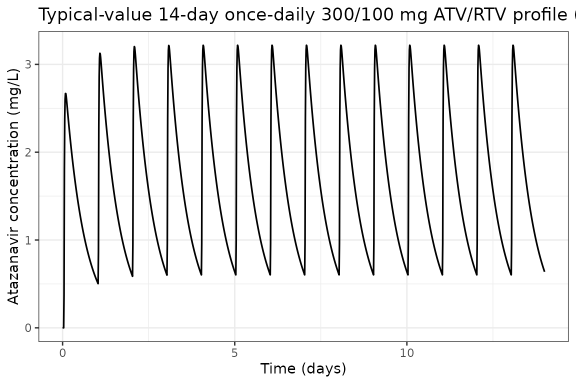
Typical-value steady-state dosing interval (Day 14, 24 h)
sim_tau <- as.data.frame(sim_ss) |>
  dplyr::filter(time >= 13 * 24, time <= 14 * 24) |>
  dplyr::mutate(t_post_dose = time - 13 * 24)

ggplot(sim_tau, aes(t_post_dose, Cc)) +
  geom_line(linewidth = 0.7) +
  labs(
    x = "Time after dose (h)",
    y = "Atazanavir concentration (mg/L)",
    title = "Typical-value steady-state dosing interval (Day 14)"
  ) +
  theme_bw()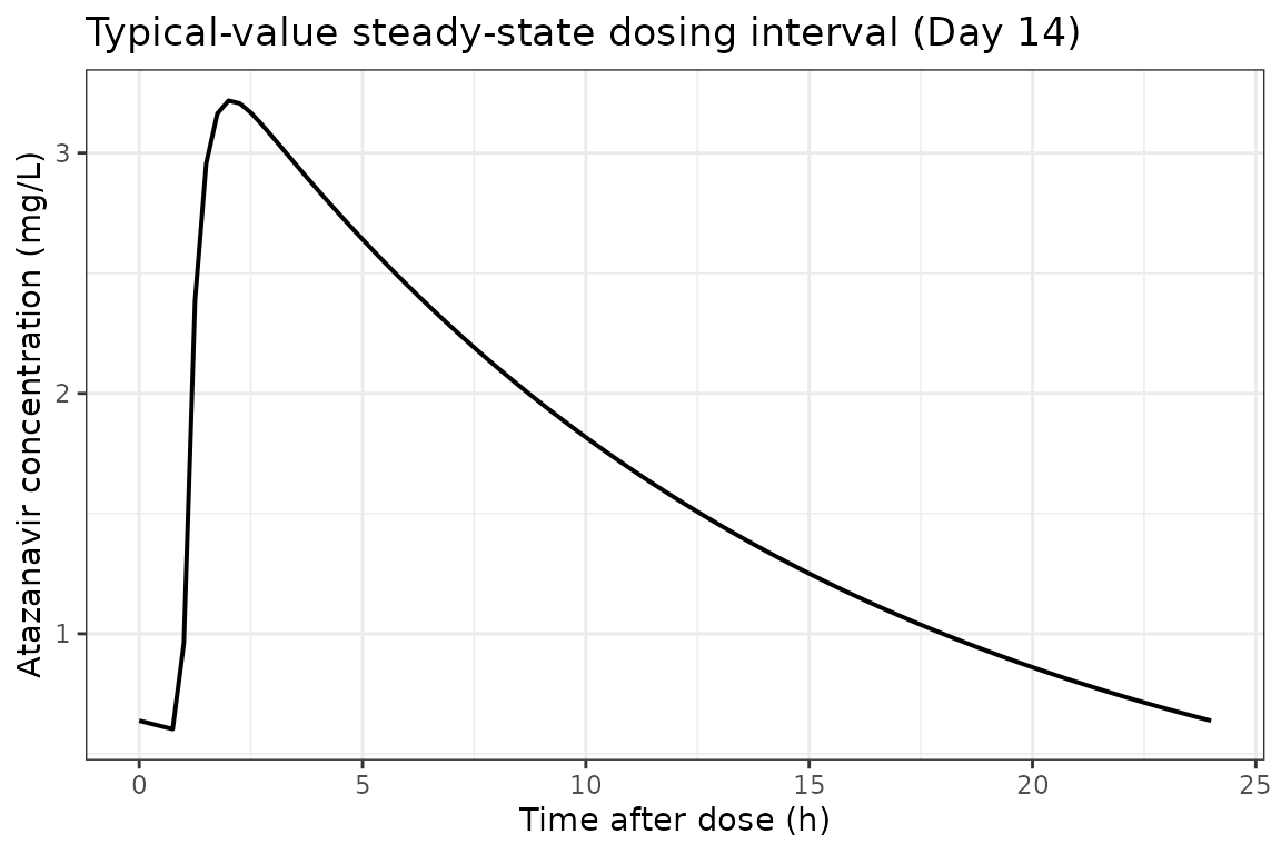
Virtual cohort matched to study demographics
We sample 80 virtual subjects whose covariate distributions reproduce the published baseline demographics. RTVAUC0-24 is sampled from approximately log-normal centred on 7.52 mg*h/L spanning the Table 1 range (2.41-22.05).
set.seed(2009)
n_subj <- 80L

# Ritonavir AUC0-24 ~ log-normal centred at the cohort median 7.52 mg*h/L,
# spanning the Table 1 range (2.41-22.05).
log_med   <- log(7.52)
log_sd    <- 0.45
CONMED_RTV_AUC   <- pmin(22.05, pmax(2.41, exp(rnorm(n_subj, log_med, log_sd))))

cohort <- data.frame(
  ID      = seq_len(n_subj),
  CONMED_RTV_AUC = CONMED_RTV_AUC
)
summary(cohort$CONMED_RTV_AUC)
#>    Min. 1st Qu.  Median    Mean 3rd Qu.    Max.
#>   2.509   5.613   7.148   8.112   9.861  22.050
Stochastic simulation across the virtual cohort
Each subject receives 14 once-daily doses; observations are at 30-min resolution during the first dosing interval and once per dose interval through Day 14.
build_subject_events <- function(id, auc_rtv) {
  ev <- rxode2::et(
    amt = 300, cmt = "depot", evid = 1,
    ii = 24, addl = 13
  ) |>
    rxode2::et(c(seq(0, 24, by = 0.5), seq(13 * 24, 14 * 24, by = 0.5))) |>
    rxode2::et(id = id)
  df <- as.data.frame(ev)
  df$CONMED_RTV_AUC <- auc_rtv
  df
}

ev_all <- do.call(
  rbind,
  Map(build_subject_events, cohort$ID, cohort$CONMED_RTV_AUC)
)

set.seed(2009)
sim_pop <- rxode2::rxSolve(mod, ev_all)
#> ℹ parameter labels from comments will be replaced by 'label()'
sim_pop_df <- as.data.frame(sim_pop)
VPC: Day-1 vs Day-14 dosing intervals
sim_day1 <- sim_pop_df |>
  filter(time >= 0, time <= 24) |>
  group_by(time) |>
  summarise(
    Q05 = quantile(ipredSim, 0.025, na.rm = TRUE),
    Q50 = quantile(ipredSim, 0.50,  na.rm = TRUE),
    Q95 = quantile(ipredSim, 0.975, na.rm = TRUE),
    .groups = "drop"
  ) |>
  mutate(panel = "Day 1")

sim_day14 <- sim_pop_df |>
  filter(time >= 13 * 24, time <= 14 * 24) |>
  mutate(time_in_panel = time - 13 * 24) |>
  group_by(time_in_panel) |>
  summarise(
    Q05 = quantile(ipredSim, 0.025, na.rm = TRUE),
    Q50 = quantile(ipredSim, 0.50,  na.rm = TRUE),
    Q95 = quantile(ipredSim, 0.975, na.rm = TRUE),
    .groups = "drop"
  ) |>
  rename(time = time_in_panel) |>
  mutate(panel = "Day 14")

vpc_df <- bind_rows(sim_day1, sim_day14)

ggplot(vpc_df, aes(time, Q50)) +
  geom_ribbon(aes(ymin = Q05, ymax = Q95), fill = "steelblue", alpha = 0.25) +
  geom_line(linewidth = 0.7) +
  facet_wrap(~panel) +
  labs(
    x = "Time after most recent dose (h)",
    y = "Atazanavir concentration (mg/L)",
    title = "Virtual-cohort VPC: median + 95% prediction interval",
    caption = "Replicates Figure 2(a) of Dickinson 2009 (300/100 mg ATV/RTV) qualitatively; the published figure is the 95% PI over 1000 simulated 24-h intervals."
  ) +
  theme_bw()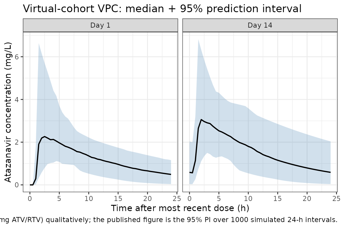
PKNCA validation
Non-compartmental analysis of the simulated steady-state (Day-14)
dosing interval. The paper does not tabulate observed Cmax / Tmax /
AUC0-24 from the NCA, but the typical-value AUC0-24 expected from
dose / CL/F = 300 / 7.7 is 38.96 mg*h/L; the Day-14
simulated cohort median should fall close to that value.
nca_concs <- sim_pop_df |>
  filter(time >= 13 * 24, time <= 14 * 24) |>
  mutate(t_in_interval = time - 13 * 24) |>
  filter(!is.na(ipredSim))

dose_records <- cohort |>
  mutate(time = 0, amt = 300) |>
  select(id = ID, time, amt)

conc_obj <- PKNCA::PKNCAconc(
  nca_concs, ipredSim ~ t_in_interval | id,
  concu = "mg/L", timeu = "h"
)
dose_obj <- PKNCA::PKNCAdose(
  dose_records, amt ~ time | id,
  doseu = "mg"
)

intervals <- data.frame(
  start    = 0,
  end      = 24,
  cmax     = TRUE,
  tmax     = TRUE,
  cmin     = TRUE,
  auclast  = TRUE,
  cav      = TRUE
)

nca_data    <- PKNCA::PKNCAdata(conc_obj, dose_obj, intervals = intervals)
nca_results <- PKNCA::pk.nca(nca_data)
nca_df      <- as.data.frame(nca_results$result)

nca_summary <- nca_df |>
  filter(PPTESTCD %in% c("cmax", "tmax", "cmin", "auclast", "cav")) |>
  group_by(PPTESTCD) |>
  summarise(
    median = median(PPORRES, na.rm = TRUE),
    P05    = quantile(PPORRES, 0.05, na.rm = TRUE),
    P95    = quantile(PPORRES, 0.95, na.rm = TRUE),
    .groups = "drop"
  )

knitr::kable(
  nca_summary, digits = 3,
  caption = "Day-14 steady-state PKNCA summary across the virtual cohort"
)| PPTESTCD | median | P05 | P95 |
|---|---|---|---|
| auclast | 38.883 | 19.354 | 70.085 |
| cav | 1.620 | 0.806 | 2.920 |
| cmax | 3.152 | 1.760 | 5.708 |
| cmin | 0.565 | 0.065 | 1.716 |
| tmax | 2.000 | 1.500 | 5.525 |
Comparison against published values
| Quantity | Paper value | Simulated (median, 5th-95th) |
|---|---|---|
| Typical AUC0-24 (mg*h/L) |
dose / CL/F = 300 / 7.7 = 38.96 mg*h/L |
nca_summary auclast median (should fall
within approximately 30-50 mg*h/L) |
| Atazanavir Cmax range (mg/L) | observed range 0.077-8.763 mg/L (538 samples) | virtual-cohort cmax 5th-95th should overlap this
range |
| Typical half-life (h) | 8.9 h (median individual estimate, Discussion) |
t1/2 = ln(2) * V/F / CL/F = 0.693 * 103 / 7.7 = 9.3 h
(typical-value algebraic) |
Dickinson 2009 does not report observed Cmax / Tmax / AUC0-24 NCA
tables in the main paper. Where the paper does report a quantitative
simulation summary (Discussion, page 1239), the model predicts 14% of
trough concentrations at 300/100 mg once daily would fall below the 0.15
mg/L viral-suppression threshold. The simulated cohort cmin
distribution above should reproduce that order of magnitude.
Assumptions and deviations
-
Lag-time IIV omitted. The paper retains a typical
lag-time of 0.96 h in the final model but reports that adding IIV on
lag-time did not improve fit (delta-OFV = -0.8; Results page 1235). The
library model follows the published final model and omits IIV on
ltlag. - Inter-laboratory error split omitted. The paper considered separate residual-error models for the two analytical laboratories and found no improvement (delta-OFV = -1.2; Results page 1235). A single combined proportional + additive residual-error model is used here.
- Ritonavir AUC0-24 supplied as a per-subject data column. The paper derives RTVAUC0-24 from observed ritonavir concentration-time data via non-compartmental analysis (WinNonlin 5.2). For simulation users without observed ritonavir concentrations, supplying the cohort median 7.52 mg*h/L reproduces typical-value behaviour. A future model could integrate the Dickinson 2008 (J Antimicrob Chemother) ritonavir PK model to compute RTVAUC0-24 endogenously.
- Concomitant medications (saquinavir, tenofovir) not modelled. Univariate tests of saquinavir and tenofovir status did not survive multivariate backwards elimination (Table 3; saquinavir significant on V/F and CL/F at p < 0.01 alone, but dropped during stepwise elimination because the model already accounted for ritonavir AUC). Body weight, sex, HIV status, and ethnicity (Black-African, Hispanic) were similarly excluded from the final model. None of these are included in the library model.
-
Log-normal IIV from reported CV%. The paper reports
IIV (%) on CL/F, V/F, and ka in the standard NONMEM exponential-model
sense. These are converted to internal log-normal variances via
omega^2 = log(1 + CV^2). - Single-laboratory assumption. The paper uses two HPLC-MS/MS laboratories that participate in the same external QA programme and shows that inter-laboratory error stratification does not improve fit (Results page 1235). The library model uses a single residual-error block.
Reference
- Dickinson L, Boffito M, Back D, Waters L, Else L, Davies G, Khoo S, Pozniak A, Aarons L. Population pharmacokinetics of ritonavir-boosted atazanavir in HIV-infected patients and healthy volunteers. J Antimicrob Chemother. 2009;63(6):1233-1243. doi:10.1093/jac/dkp102