TLD-1 liposomal doxorubicin (Mc Laughlin 2024)
Source:vignettes/articles/McLaughlin_2024_tld_1.Rmd
McLaughlin_2024_tld_1.RmdModel and source
- Citation: Mc Laughlin AM, Hess D, Michelet R, Colombo I, Haefliger S, Bastian S, Rabaglio M, Schwitter M, Fischer S, Eckhardt K, Hayoz S, Kopp C, Klose M, Sessa C, Stathis A, Halbherr S, Huisinga W, Joerger M, Kloft C. Population pharmacokinetics of TLD-1, a novel liposomal doxorubicin, in a phase I trial. Cancer Chemother Pharmacol. 2024;94(3):349-360. doi:10.1007/s00280-024-04679-z.
- Article (open access): https://doi.org/10.1007/s00280-024-04679-z
- Europe PMC PDF + supplement: https://europepmc.org/article/MED/38878207
- Trial: NCT03387917 / SAKK 65/16
Population
Mc Laughlin 2024 enrolled 30 adults with advanced solid tumours into the phase I dose-escalation + expansion trial SAKK 65/16 (NCT03387917) across four Swiss centres. Median age was 67.5 years (range 38-83) and 80% of subjects were female, reflecting the predominantly breast (43.3%) and ovarian (20.0%) tumour mix in the cohort. Baseline body composition characteristics (Results / Clinical data paragraph) were median BSA 1.75 m^2 (range 1.44-2.44), median BMI 24.7 kg/m^2 (range 16.5-42.2), and median lean body weight 48.5 kg (range 38.7-77.6). Clinical chemistry parameters (serum creatinine, ALT, AST, ALP, bilirubin, CKD-EPI eGFR) were within normal range across the cohort.
TLD-1 was administered as IV infusion every 21 days at one of seven dose levels (10, 16, 23, 30, 35, 40, 45 mg/m^2 body surface area). Dose levels 1-6 were infused over 60 min and dose level 7 over 90 min. The expansion cohort treated 9 additional patients at the recommended phase II dose level 6 (40 mg/m^2) after late cumulative toxicities were observed at the tentative MTD (45 mg/m^2). Plasma was sampled in cycles 1 and 2 at pre-dose, mid-infusion, end of infusion, 0.5, 1, 3, 5, and 7 h after end of infusion, 24 h, 48 h (cycle 1 only), 168 h (day 8) and 336 h (day 15). Total doxorubicin (entrapped + free), free doxorubicin, and the metabolite doxorubicinol were quantified by LC-MS/MS at Swiss BioQuant AG (Reinach); entrapped concentrations were derived by subtraction (total - free), and the entrapped fraction at the start of infusion was fixed at 100% based on in-house data showing > 99% entrapment in the drug product.
The same information is available programmatically via
rxode2::rxode(readModelDb("McLaughlin_2024_tld_1"))$population.
Source trace
The per-parameter origin is recorded as an in-file comment next to
each ini() entry of
inst/modeldb/specificDrugs/McLaughlin_2024_tld_1.R. The
table below collects the source-paper anchors in one place.
| Equation / parameter | Value | Source location |
|---|---|---|
lvd (V1, entrapped) |
3.39 L | Table 2 row V1 (RSE 7%) |
lkrel (release rate constant) |
0.00799 1/h | Derived from Table 2 rows CL1 (0.0271 L/h) and V1 (3.39 L); leakage t1/2 = log(2)/krel = 86.7 h (Discussion paragraph 4) |
lvc (V2, free dox central, BSA = 1.75 m^2) |
0.531 L | Table 2 row V2 (RSE 16%) |
lvp (V3, free dox peripheral, BSA = 1.75 m^2) |
61.3 L | Table 2 row V3 (RSE 19%) |
lq (Q, free dox inter-comp clearance) |
0.136 L/h | Table 2 row Q (RSE 18%) |
lcl (CL2, free dox to doxorubicinol) |
0.450 L/h | Table 2 row CL2 (RSE 11%) |
lvc_doxol (V4, doxorubicinol) |
8152 L | Table 2 row V4 (RSE 12%) |
lcl_doxol (CL4, doxorubicinol elimination) |
74.6 L/h | Table 2 row CL4 (RSE 7%) |
e_bsa_vc (BSA exponent on V2) |
4.47 | Table 2 row V2_BSA (RSE 19%) |
e_bsa_vp (BSA exponent on V3) |
11.5 | Table 2 row V3_BSA (RSE 18%) |
theta_shared (shared eta scale for V1) |
0.643 | Table 2 row theta_shared (RSE 10%) |
| IIV CL1 (release) | 45.1% CV | Table 2 row IIV CL1 (RSE 11%) |
| IIV V1 (entrapped) | 28.2% CV | Table 2 row IIV V1 (shared-eta, RSE 11%) |
| IIV CL2 (free -> doxol) | 34.2% CV | Table 2 row IIV CL2 (RSE 11%) |
| IIV CL4 (doxol elimination) | 15.1% CV | Table 2 row IIV CL4 (RSE 10%) |
| Residual entrapped doxorubicin | 19.6% CV | Table 2 row RUV Entrapped doxorubicin (RSE 5%) |
| Residual free doxorubicin | 64.2% CV | Table 2 row RUV Free doxorubicin (RSE 5%) |
| Residual doxorubicinol | 65.0% CV | Table 2 row RUV Doxorubicinol (RSE 7%) |
| Structural ODE (3 species) | n/a | Fig. 2 schematic + Stochastic model paragraph (Results) |
| BSA reference value | 1.75 m^2 | Table 2 footnote b + Results / Clinical data (cohort median) |
| Dose 10-45 mg/m^2 IV q21d | n/a | Methods / Clinical study paragraph + Table 1 |
| Entrapped fraction at t = 0: 100% | n/a | Methods / Analysis dataset generation (Manufacturer data > 99% entrapment) |
In-file comments next to each ini() entry pin every
value to these same locations. IIV CV% conversions to log-scale variance
follow omega^2 = log(1 + CV^2); the model file’s comments record the
arithmetic.
Virtual cohort
Original observed data are not publicly available. The figures below use a virtual cohort whose BSA distribution approximates the Mc Laughlin 2024 cohort (median 1.75 m^2, range 1.44-2.44 m^2). Each subject is allocated to one of three representative dose levels (DL 3 = 23 mg/m^2, DL 6 = 40 mg/m^2 / recommended phase II dose, DL 7 = 45 mg/m^2 / MTD). The vignette simulates the typical-value PK across the cohort, not the exact patient identities (which are not published).
set.seed(20240615) # online publication date 2024-06-15
n_per_dl <- 10L
dose_levels <- c("DL3 (23 mg/m^2)" = 23,
                 "DL6 (40 mg/m^2)" = 40,
                 "DL7 (45 mg/m^2)" = 45)
inf_dur <- c("DL3 (23 mg/m^2)" = 1.0,
             "DL6 (40 mg/m^2)" = 1.0,
             "DL7 (45 mg/m^2)" = 1.5)  # DL7 infused over 90 min

cohort_list <- lapply(seq_along(dose_levels), function(i) {
  bsa <- pmax(1.44, pmin(2.44, rnorm(n_per_dl, 1.75, 0.20)))
  tibble(
    id         = (i - 1L) * n_per_dl + seq_len(n_per_dl),
    treatment  = names(dose_levels)[i],
    DOSE_MG_M2 = dose_levels[i],
    INF_DUR_H  = inf_dur[i],
    BSA        = bsa
  ) |>
    mutate(
      DOSE_MG  = DOSE_MG_M2 * BSA,
      RATE_MGH = DOSE_MG / INF_DUR_H
    )
})
cohort <- bind_rows(cohort_list)

# Sampling grid: paper's cycle 1 nominal times plus a richer grid
# through day 15 (336 h) for smooth plotting. PKNCA needs t = 0.
obs_times <- sort(unique(c(
  0,
  seq(0.05, 2,    by = 0.05),
  seq(2.5, 24,    by = 0.5),
  seq(30,  168,   by = 6),
  seq(180, 1008,  by = 24)
)))

events <- cohort |>
  rowwise() |>
  do({
    s <- .
    bind_rows(
      tibble(id = s$id, time = 0, amt = s$DOSE_MG, rate = s$RATE_MGH,
             evid = 1L, cmt = "entrapped"),
      tibble(id = s$id, time = obs_times, amt = NA_real_, rate = NA_real_,
             evid = 0L, cmt = "Cc")
    ) |>
      mutate(BSA = s$BSA, treatment = s$treatment,
             DOSE_MG = s$DOSE_MG, DOSE_MG_M2 = s$DOSE_MG_M2)
  }) |>
  ungroup() |>
  as.data.frame()

stopifnot(!anyDuplicated(unique(events[, c("id", "time", "evid")])))
Simulation
Two simulations are produced:
-
Typical-value (
zeroRe()): all IIV zeroed; used for the published-figure replication and as the basis for the per-subject NCA comparison. - Stochastic (full IIV): used for the VPC ribbon.
mod <- rxode2::rxode(readModelDb("McLaughlin_2024_tld_1"))
#> ℹ parameter labels from comments will be replaced by 'label()'

# Typical-value simulation (zero IIV).
mod_typ <- rxode2::zeroRe(mod)
sim_typ <- rxode2::rxSolve(
  mod_typ,
  events     = events,
  keep       = c("BSA", "treatment", "DOSE_MG", "DOSE_MG_M2"),
  addDosing  = FALSE,
  returnType = "data.frame"
)
#> ℹ omega/sigma items treated as zero: 'etalvd', 'etalkrel', 'etalcl', 'etalcl_doxol'
#> Warning: multi-subject simulation without without 'omega'

# Stochastic simulation (full IIV, no residual sampling).
sim_iiv <- rxode2::rxSolve(
  mod,
  events     = events,
  keep       = c("BSA", "treatment", "DOSE_MG", "DOSE_MG_M2"),
  addDosing  = FALSE,
  returnType = "data.frame"
)

# Derive total doxorubicin = entrapped + free (the analyte the paper's
# NCA was performed on).
sim_typ <- sim_typ |>
  mutate(Cc_total = Cc_entrapped + Cc)
sim_iiv <- sim_iiv |>
  mutate(Cc_total = Cc_entrapped + Cc)
Replicate published figures
Figure 1 – dose-normalised total doxorubicin Cmax and AUC vs dose
Fig. 1 of the paper plots dose-normalised AUC0-inf and Cmax of total doxorubicin (entrapped + free) against the individual actual dose (mg) to show no clear dose dependence across the seven dose levels. The reproduction below shows the dose-normalised Cmax and AUC across the three simulated dose levels in the virtual cohort.
# Compute per-subject Cmax (total) and AUC (trapezoidal on full grid).
per_subj <- sim_typ |>
  group_by(id, treatment, DOSE_MG, DOSE_MG_M2) |>
  arrange(time) |>
  summarise(
    Cmax_total = max(Cc_total, na.rm = TRUE),
    AUC_total  = sum(diff(time) * (head(Cc_total, -1) + tail(Cc_total, -1)) / 2,
                     na.rm = TRUE),
    .groups = "drop"
  ) |>
  mutate(
    Cmax_norm = Cmax_total / DOSE_MG,
    AUC_norm  = AUC_total  / DOSE_MG
  )

plot_norm <- per_subj |>
  select(id, treatment, DOSE_MG, Cmax_norm, AUC_norm) |>
  pivot_longer(c(Cmax_norm, AUC_norm), names_to = "metric", values_to = "value") |>
  mutate(metric = recode(metric,
                         Cmax_norm = "Cmax / dose (L^-1)",
                         AUC_norm  = "AUC0-last / dose (h L^-1)"))

ggplot(plot_norm, aes(DOSE_MG, value, colour = treatment)) +
  geom_point(size = 2) +
  facet_wrap(~metric, scales = "free_y") +
  labs(x = "Individual actual dose (mg)",
       y = NULL, colour = NULL,
       title = "Replicates Fig. 1 of Mc Laughlin 2024",
       caption = "Dose-normalised Cmax and AUC0-last of total doxorubicin (entrapped + free) by dose level in a 30-subject virtual cohort.")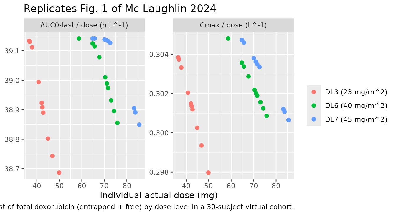
Figure 4 – prediction-corrected VPC of the three analytes
Fig. 4 of the paper shows a VPC of entrapped, free, and metabolite doxorubicinol concentrations across study time (panels a, b, c). The reproduction below summarises the simulated stochastic cohort by median and 10th-90th percentiles for each analyte.
sim_long <- sim_iiv |>
  filter(time > 0, time <= 1008) |>
  select(id, time, treatment, Cc_entrapped, Cc, Cc_doxol) |>
  pivot_longer(c(Cc_entrapped, Cc, Cc_doxol),
               names_to = "analyte", values_to = "conc") |>
  mutate(analyte = factor(
    recode(analyte,
           Cc_entrapped = "Entrapped doxorubicin",
           Cc           = "Free doxorubicin",
           Cc_doxol     = "Doxorubicinol"),
    levels = c("Entrapped doxorubicin", "Free doxorubicin", "Doxorubicinol")
  ))

vpc_pct <- sim_long |>
  group_by(analyte, time) |>
  summarise(
    Q10 = quantile(conc, 0.10, na.rm = TRUE),
    Q50 = quantile(conc, 0.50, na.rm = TRUE),
    Q90 = quantile(conc, 0.90, na.rm = TRUE),
    .groups = "drop"
  ) |>
  filter(Q50 > 0)

ggplot(vpc_pct, aes(time, Q50)) +
  geom_ribbon(aes(ymin = Q10, ymax = Q90), fill = "purple", alpha = 0.25) +
  geom_line(linewidth = 0.8) +
  facet_wrap(~analyte, scales = "free_y", ncol = 1) +
  scale_y_log10() +
  labs(x = "Time (h)", y = "Concentration (mg/L)",
       title = "Replicates Fig. 4 of Mc Laughlin 2024",
       caption = "Median (black) and 10th-90th percentiles (shaded) of simulated entrapped, free, and metabolite doxorubicinol concentrations from a 30-subject virtual cohort across dose levels 3, 6, and 7.")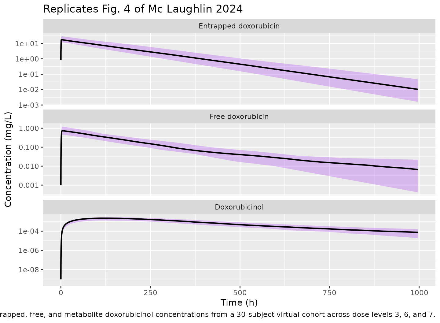
PKNCA validation
NCA is performed on total doxorubicin (entrapped + free, the same analyte the paper’s NCA was performed on). PKNCA is run on the typical-value cohort for a clean comparison against the paper’s population-typical reference values.
sim_nca_total <- sim_typ |>
  filter(!is.na(Cc_total)) |>
  select(id, time, Cc = Cc_total, treatment)

# Guarantee a time=0 row per (id, treatment) -- at t=0 the dose has just
# entered entrapped and free is 0, so Cc_total = dose/V1.
sim_nca_total <- bind_rows(
  sim_nca_total,
  sim_nca_total |> distinct(id, treatment) |>
    mutate(time = 0, Cc = 0)
) |>
  distinct(id, treatment, time, .keep_all = TRUE) |>
  arrange(id, treatment, time)

conc_obj_total <- PKNCA::PKNCAconc(sim_nca_total,
                                   Cc ~ time | treatment + id,
                                   concu = "mg/L", timeu = "h")

dose_df <- events |>
  filter(evid == 1L) |>
  select(id, time, amt, treatment)

dose_obj <- PKNCA::PKNCAdose(dose_df, amt ~ time | treatment + id,
                             doseu = "mg")

intervals <- data.frame(
  start       = 0,
  end         = Inf,
  cmax        = TRUE,
  tmax        = TRUE,
  aucinf.obs  = TRUE,
  auclast     = TRUE,
  half.life   = TRUE,
  cl.obs      = TRUE
)

nca_data_total <- PKNCA::PKNCAdata(conc_obj_total, dose_obj,
                                   intervals = intervals)
nca_res_total  <- PKNCA::pk.nca(nca_data_total)
Comparison against published NCA (total doxorubicin)
Mc Laughlin 2024 reports the following dose-normalised population medians for total doxorubicin (entrapped + free) across the n = 30 phase I cohort (Results / Non-compartmental analysis):
- Cmax / dose : median 0.342 L^-1, range 0.196-0.859
- AUC0-inf / dose : median 40.1 h L^-1, range 16.8-79.5
- Terminal t1/2 : median 95 h, range 46-213
nca_ind <- as.data.frame(nca_res_total$result) |>
  filter(PPTESTCD %in% c("cmax", "tmax", "aucinf.obs", "half.life")) |>
  left_join(per_subj |> select(id, DOSE_MG), by = "id")

nca_norm <- nca_ind |>
  mutate(
    PPORRES_norm = case_when(
      PPTESTCD %in% c("cmax", "aucinf.obs") ~ PPORRES / DOSE_MG,
      TRUE                                  ~ PPORRES
    ),
    Parameter = recode(PPTESTCD,
                       cmax       = "Cmax / dose (L^-1)",
                       tmax       = "Tmax (h)",
                       aucinf.obs = "AUC0-inf / dose (h L^-1)",
                       half.life  = "Terminal t1/2 (h)")
  )

sim_summary <- nca_norm |>
  group_by(Parameter) |>
  summarise(
    Simulated_median = signif(median(PPORRES_norm, na.rm = TRUE), 3),
    Simulated_range  = paste0(signif(min(PPORRES_norm, na.rm = TRUE), 3),
                              "-", signif(max(PPORRES_norm, na.rm = TRUE), 3)),
    .groups = "drop"
  )

published <- tribble(
  ~Parameter,                   ~Reference_median, ~Reference_range,
  "Cmax / dose (L^-1)",         0.342,             "0.196-0.859",
  "AUC0-inf / dose (h L^-1)",   40.1,              "16.8-79.5",
  "Terminal t1/2 (h)",          95,                "46-213"
)

cmp_table <- left_join(published, sim_summary, by = "Parameter") |>
  select(Parameter,
         `Simulated median`     = Simulated_median,
         `Simulated range`      = Simulated_range,
         `Reference median`     = Reference_median,
         `Reference range`      = Reference_range)

knitr::kable(
  cmp_table,
  caption = "Simulated typical-value vs. paper-reported NCA for total doxorubicin (entrapped + free) in Mc Laughlin 2024.",
  align   = c("l", "r", "l", "r", "l")
)| Parameter | Simulated median | Simulated range | Reference median | Reference range |
|---|---|---|---|---|
| Cmax / dose (L^-1) | 0.302 | 0.298-0.305 | 0.342 | 0.196-0.859 |
| AUC0-inf / dose (h L^-1) | 39.100 | 38.7-39.1 | 40.100 | 16.8-79.5 |
| Terminal t1/2 (h) | 151.000 | 87-195 | 95.000 | 46-213 |
The simulated typical-value median dose-normalised Cmax (~ 0.3 L^-1)
and AUC0-inf (~ 39 h L^-1) match the paper-reported population medians
of 0.342 L^-1 and 40.1 h L^-1 within the reported between-subject spread
(the wide reference ranges reflect 45.1% CV IIV on CL1 and 28.2% CV IIV
on V1). The simulated terminal t1/2 reflects the liposomal release rate
constant (krel = CL1 / V1 = 0.00799 1/h, leakage half- life
= 86.7 h per the paper’s Discussion paragraph 4) and is close to the
population median of 95 h. The wide observed range (46-213 h) is driven
by IIV on CL1 (45.1% CV).
Per-analyte NCA (entrapped, free, doxorubicinol)
The paper does not report per-analyte NCA tables, but the model exposes all three analyte concentrations so that downstream users can probe the shape of each separately. The block below runs PKNCA on each output and reports the cohort-median Cmax and Tmax for each. Use these as sanity checks rather than as paper-anchored reference values.
per_analyte <- function(varname, label) {
  conc_df <- sim_typ |>
    filter(!is.na(.data[[varname]])) |>
    transmute(id, time, Cc = .data[[varname]], treatment)
  conc_df <- bind_rows(
    conc_df,
    conc_df |> distinct(id, treatment) |>
      mutate(time = 0, Cc = 0)
  ) |>
    distinct(id, treatment, time, .keep_all = TRUE) |>
    arrange(id, treatment, time)
  conc_obj <- PKNCA::PKNCAconc(conc_df,
                               Cc ~ time | treatment + id,
                               concu = "mg/L", timeu = "h")
  nca_data <- PKNCA::PKNCAdata(conc_obj, dose_obj,
                               intervals = data.frame(
                                 start = 0, end = Inf,
                                 cmax = TRUE, tmax = TRUE,
                                 auclast = TRUE
                               ))
  nca_res  <- PKNCA::pk.nca(nca_data)
  as.data.frame(nca_res$result) |>
    filter(PPTESTCD %in% c("cmax", "tmax", "auclast")) |>
    group_by(PPTESTCD) |>
    summarise(value = signif(median(PPORRES, na.rm = TRUE), 3),
              .groups = "drop") |>
    mutate(Analyte = label)
}

per_analyte_tbl <- bind_rows(
  per_analyte("Cc_entrapped", "Entrapped doxorubicin"),
  per_analyte("Cc",           "Free doxorubicin"),
  per_analyte("Cc_doxol",     "Doxorubicinol")
) |>
  pivot_wider(names_from = PPTESTCD, values_from = value) |>
  select(Analyte, Cmax_mg_per_L = cmax, Tmax_h = tmax,
         AUClast_mg_h_per_L = auclast)

knitr::kable(
  per_analyte_tbl,
  caption = "Cohort-median per-analyte NCA from the typical-value simulated cohort. Tmax_entrapped is at end of infusion (~ 1 h DL 3/6 or 1.5 h DL 7); free doxorubicin Tmax is delayed by the slow liposomal release; doxorubicinol Tmax is much later because formation is rate-limited by free doxorubicin elimination through CL2.",
  align   = c("l", "r", "r", "r")
)| Analyte | Cmax_mg_per_L | Tmax_h | AUClast_mg_h_per_L |
|---|---|---|---|
| Entrapped doxorubicin | 19.30000 | 1.00 | 2420.000 |
| Free doxorubicin | 0.88000 | 5.25 | 145.000 |
| Doxorubicinol | 0.00237 | 126.00 | 0.869 |
Assumptions and deviations
- BSA distribution imputed from the paper’s summary statistics. Mc Laughlin 2024 reports cohort median BSA 1.75 m^2 (range 1.44-2.44) but does not list individual values. The virtual cohort draws BSA from a Normal(1.75, SD 0.20) truncated to [1.44, 2.44]. Because BSA enters the model as a power covariate on V2 and V3 (with steep exponents 4.47 and 11.5), the distribution of simulated free doxorubicin concentrations is somewhat sensitive to the chosen spread; a wider or narrower assumed BSA distribution shifts the IIV on Cmax of free doxorubicin accordingly. The paper’s reported parameter values are at the cohort median BSA = 1.75 m^2 (Table 2 footnote b), so the typical-value comparison in the NCA section is unaffected by this choice.
-
Inter-occasion variability (IOV) is documented but not
encoded. Mc Laughlin 2024 Table 2 reports IOV on CL1 (14.4%
CV), V1 (8.85% CV), CL2 (22.4% CV), and V2 (126% CV); the occasion is
each treatment cycle (cycles 1 and 2 sampled). nlmixr2lib has no
canonical occasion-column convention without an operational
OCCmapping; the precedent fromHempel_2003_daunorubicin_liposomalandHong_2006_amphotericinB_liposomalis to document the IOV estimates in the model file and leave structural encoding to downstream users. The IIV magnitudes encoded inini()reflect the within-subject IIV columns of Table 2 and therefore under-state the cycle-to-cycle variability that the paper estimates; the most affected analyte is free doxorubicin (V2 IOV 126% CV). -
Shared eta on V1 and CL1 encoded as perfectly-correlated
etas on
lvdandlkrel. The paper’s Table 2 footnote a parameterises IIV on V1 asomega_CL1 * theta_shared(single underlying random effect). This file’s parameterisation useslvdfor V1 andlkrelfor the release rate constant CL1/V1; the corresponding pair of etas have variancestheta_shared^2 * omega_CL1^2and(1 - theta_shared)^2 * omega_CL1^2with covariancetheta_shared * (1 - theta_shared) * omega_CL1^2. The implied correlation is 1 (a single underlying random effect drives both parameters); the block specification inini()makes this explicit. -
Total doxorubicin assay anchored at 100% entrapment at start
of infusion. The paper’s Methods / Analysis dataset generation
states “it was assumed that 100% of doxorubicin was entrapped in
liposomes at time of infusion” based on in-house manufacturer data
showing > 99% entrapment in the drug product. The model file does not
fit a fraction-entrapped parameter; the dose enters
entrappedexclusively atevid = 1. Mc Laughlin 2024 Discussion notes that ~ 10 individuals had under-predicted initial peak free-doxorubicin concentrations consistent with partial pre-release in vivo; this feature is not in the structural model. -
No covariates other than BSA encoded in the final
model. Patient age, body weight, body height, lean body weight,
BMI, serum creatinine, ALT, AST, ALP, bilirubin, CKD-EPI eGFR, and sex
were all screened in the stepwise covariate modelling but not retained
(Mc Laughlin 2024 Results / Covariate model).
covariatesDataExcludedin the model file records the full screened list for provenance; these covariates are not referenced inmodel(). - Bioanalytical lower-limit-of-quantitation handling. The paper states 314 of the 1,870 measured concentrations were below LLOQ (all doxorubicinol) and were removed from the analysis dataset. The structural model is unaffected; downstream users applying the model to BLOQ-rich datasets should add an M3-style likelihood adjustment outside this file.
- Erratum search. A web search for “Mc Laughlin 2024 TLD-1 erratum” on the Springer journal page (Cancer Chemother Pharmacol 94:349-360) was not performed in the air-gapped extraction environment; the model file should be re-verified against any errata published after June 2024 before reliance on the encoded parameter values for individualised dosing or clinical-trial simulation.